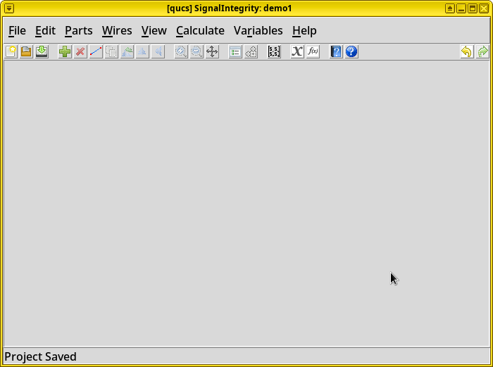
Transient Analysis via SignalIntegrity
This tutorial has repeatedly claimed that the frequency response is all you need: Once the DUT’s S-parameters are known, linear circuit analysis tools can evaluate its behavior under other input signals, so there’s no loss of generality. In fact, performing a time-domain transient simulation using frequency-domain S-parameters is a common feature in many proprietary commercial circuit simulators, such as HyperLynx, ADS, or AWR. A third-party tool also exists for PSpice. [4]_
However, in the free and open source world, few (if any) free and open source circuit simulators have this capability. For example, Ngspice supports S-parameter calculation but not transient simulation. [5]_ Qucs, too, doesn’t support transient simulation with S-parameters, although it’s possible to define devices using them.
The Python package SignalIntegrity, designed for signal integrity and eye diagram simulations from the ground up, is a rare exception. It’s developed by Pete Pupalaikis, a former signal integrity expert at LeCroy.
See also
Book. The software’s internal theory of operation is also published almost in full in the textbook S-Parameters for Signal Integrity [6]_. Each concept is accomplished by both formulas and executable code, making it an invaluable reference in this field. The author of this tutorial recommends everyone who simulates or measures RF/microwave devices to get a copy.
PyBERT. It’s another circuit simulator designed with time-domain S-parameter simulation and signal integrity in mind, developed by David Banas. See [23]_.
Install
To install SignalIntegrity, download the latest .zip file
at the project’s release page using a Web browser:
https://github.com/Nubis-Communications/SignalIntegrity/releases
As of writing, the latest version was 1.4.1. Once downloaded, unzip the file and install it locally via pip:
unzip SignalIntegrity-1.4.1.zip
cd SignalIntegrity-1.4.1

pip3 install . --user
SignalIntegrity is both a software library and a Tcl/Tk (Tkinter)
GUI application, installed to ~/.local/bin/ (or another standard
local path). You should be able to start it via:
$ SignalIntegrity
If not, you may need to add this local bin directory into
your shell’s search path.
The classic 1990s Tcl/Tk (Tkinter) GUI may look old-fashioned, but it works, and will keep working until the end of time.
Impulse Signal Analysis
For the first example, let’s examine the circuit’s time-domain response to a short impulse.
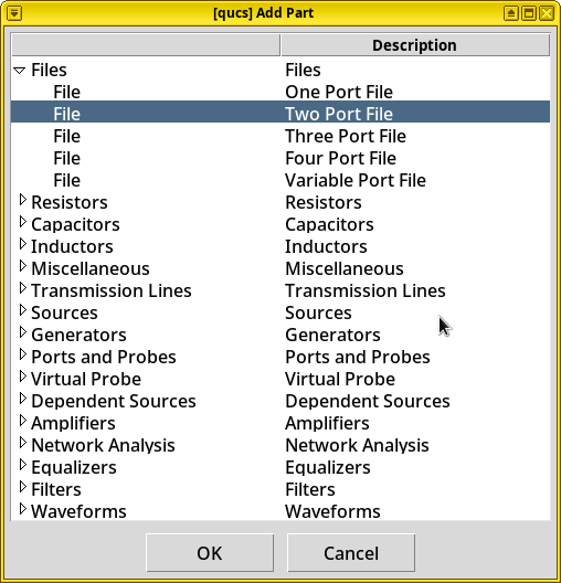
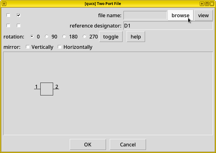
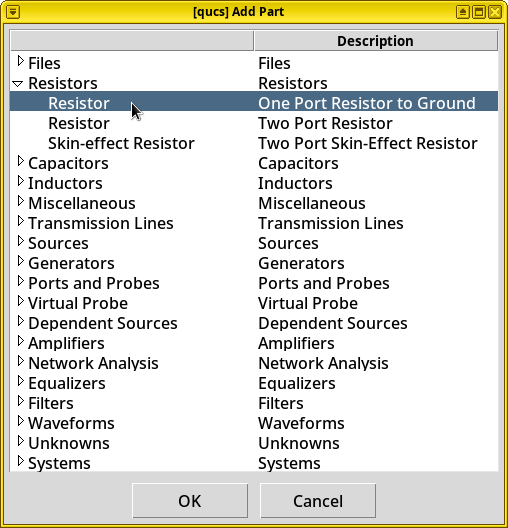
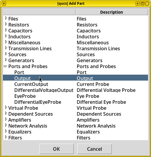
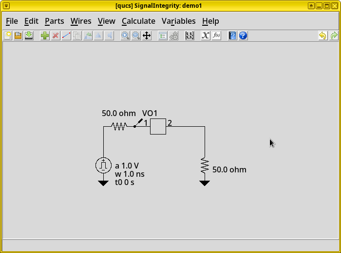
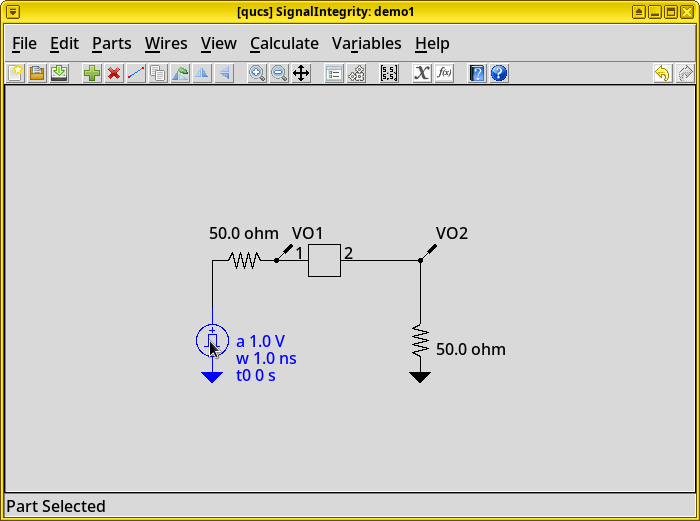
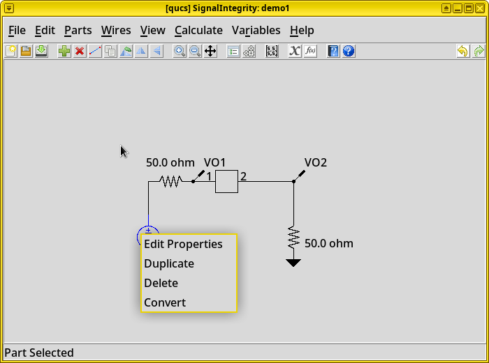
Add an S-parameter defined 2-port network. Right click on the
empty schematic, choose Add Part. In the Add
Part diagram, click . In
the opened setting window, click
browse and select the s2p S-parameter file created
by our simulation. Click OK, and finally click the empty
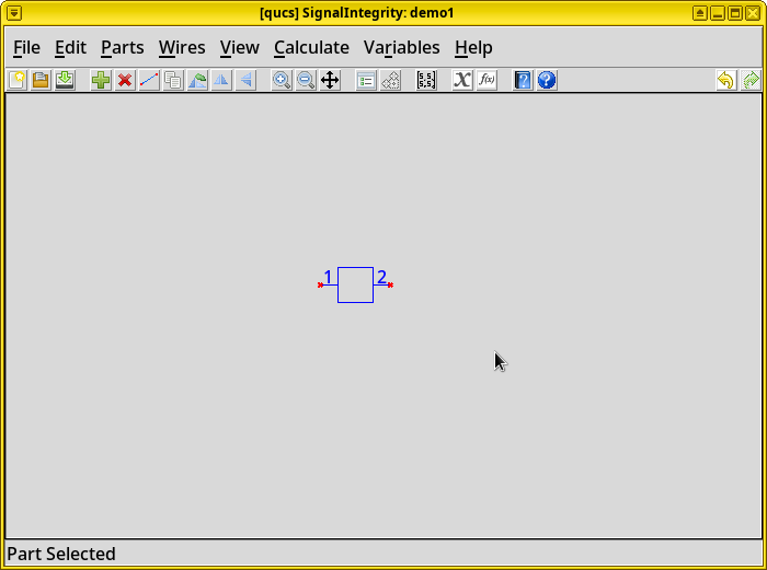
schematic to place the item. The item can be moved by selecting it
and dragging it.
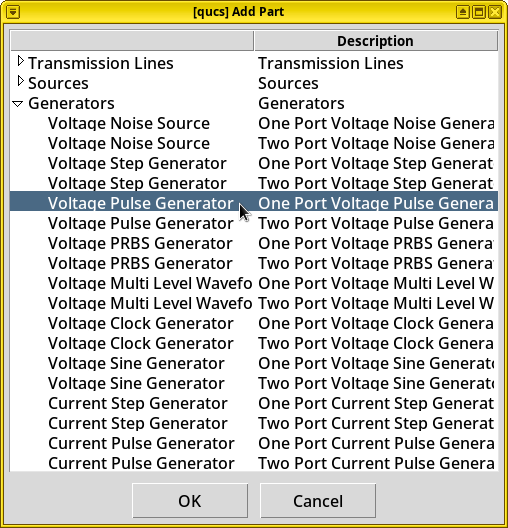
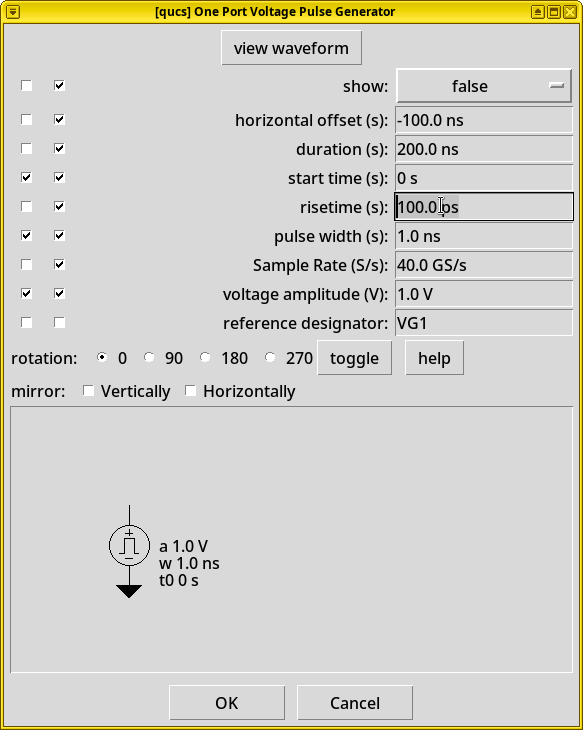
Add a voltage pulse generator. In the Add Part dialog, choose . In the opened setting window, change the risetime (s) property to “100 ps”, and place this item on the schematic.
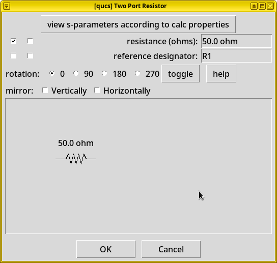
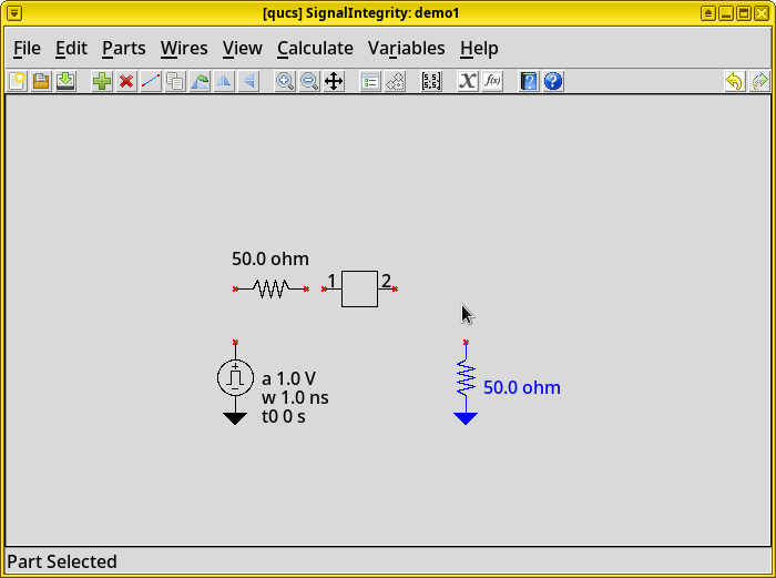
Add a series resistor to represent the generator’s output impedance. In the Add Part dialog, choose . Place this item on the schematic.
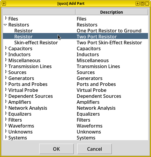
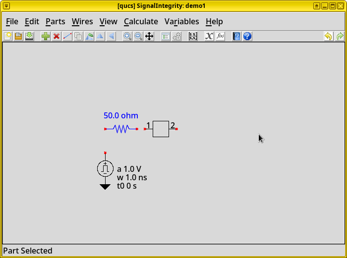
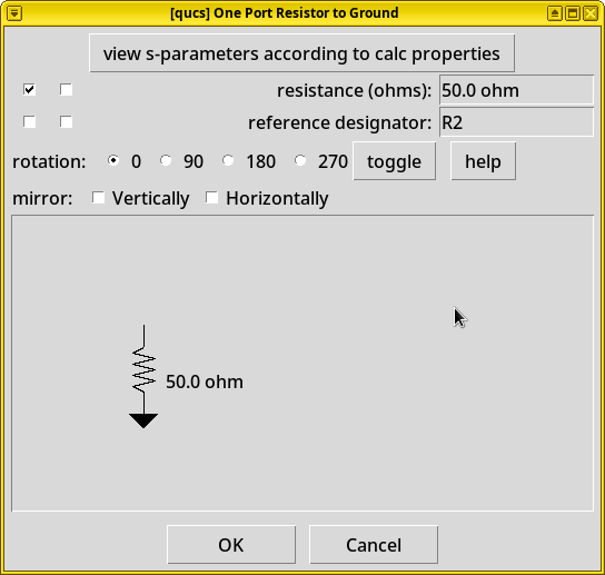
Add a resistor to ground to represent the input impedance at the end of the waveguide. In the Add Part dialog, choose . Place this item on the schematic.
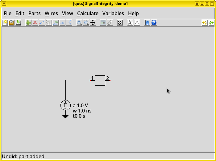
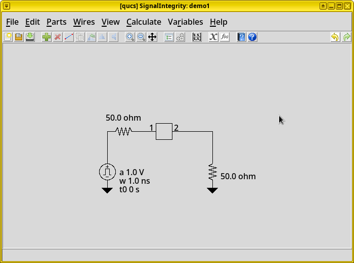
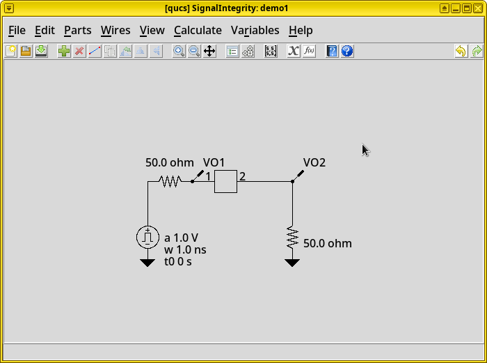
Wire the circuit. Right click on the schematic, choose Add Wire, connect the components following this order: pulse generator, series resistor, DUT Port 1, DUT Port 2, resistor to ground.
Add an input probe. In the Add Part window, choose . Place this probe on the wire after the series resistor at the DUT Port 1.
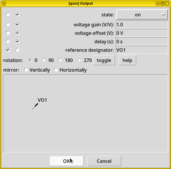
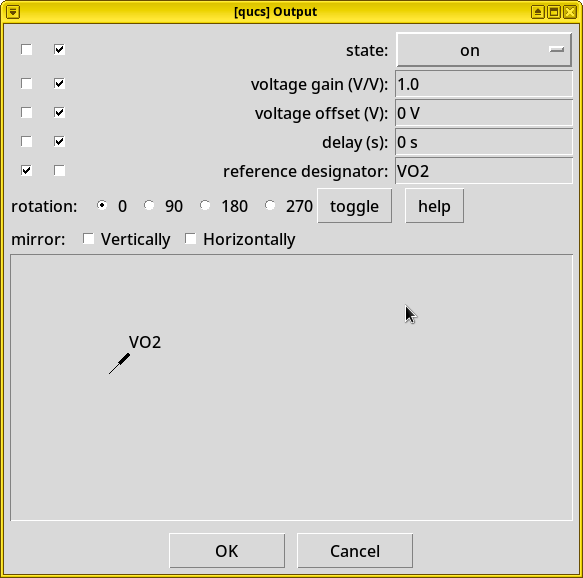
Add an output probe. Repeat the above step, add another probe on top (in parallel) of the resistor to ground, at the DUT Port 2.
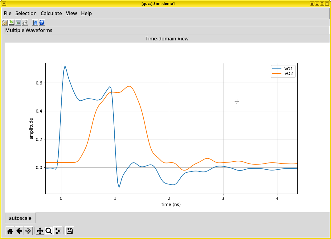
Run simulation. Click Calculate on the menu bar, and choose Simulate. After simulation finishes, it opens a time-domain line chart. After pressing the “Zoom” (magnifying glass) button and dragging a rectangle on a part of the waveform of interest, one can finally see the pulse response of the DUT.
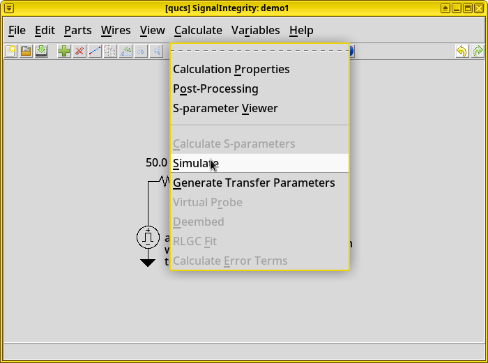
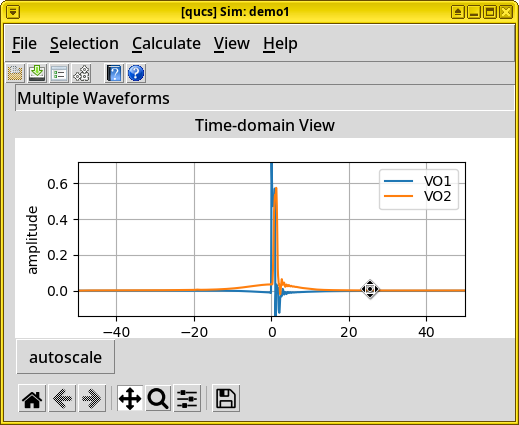
Results. As expected, the +/- 1 V input signal (+/- 0.5 V with 50 Ω output and input impedance) has severe overshoots and undershoots due to port impedance mismatches, while the output shows significant rise time degradation due to high insertion loss above 2 GHz.
Eye Diagram Analysis
For the next example, let’s examine the circuit’s time-domain signal integrity using a Pseudo-Random Bit Stream (PRBS) generator as the input, and to plot its output on an eye diagram.
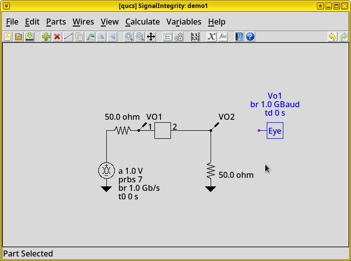
Delete the voltage pulse generator. Right-click the voltage pulse generator we added previously, select delete.
Important
Don’t select convert, it seems buggy and would prevent the generation of eye diagram after simulation.
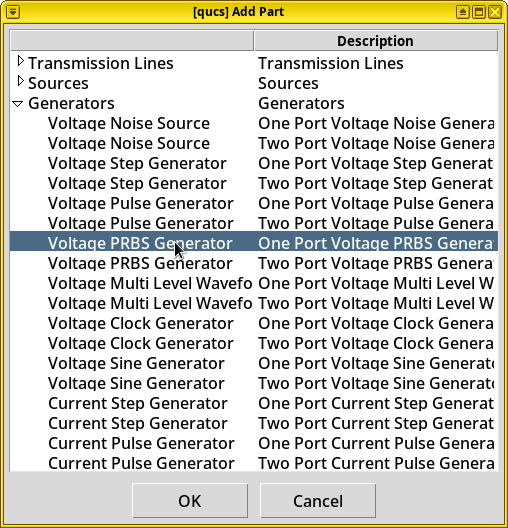
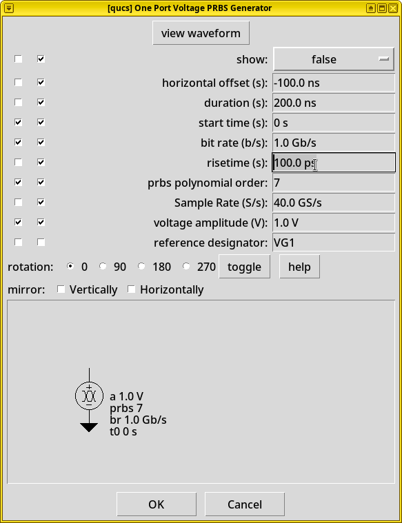
Add a Pseudo-Random Bitstream Generator (PSBG). In the Add Part dialog, choose . Change its risetime (s) to “100 ps”. Place this item on the schematic.
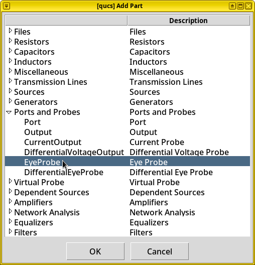
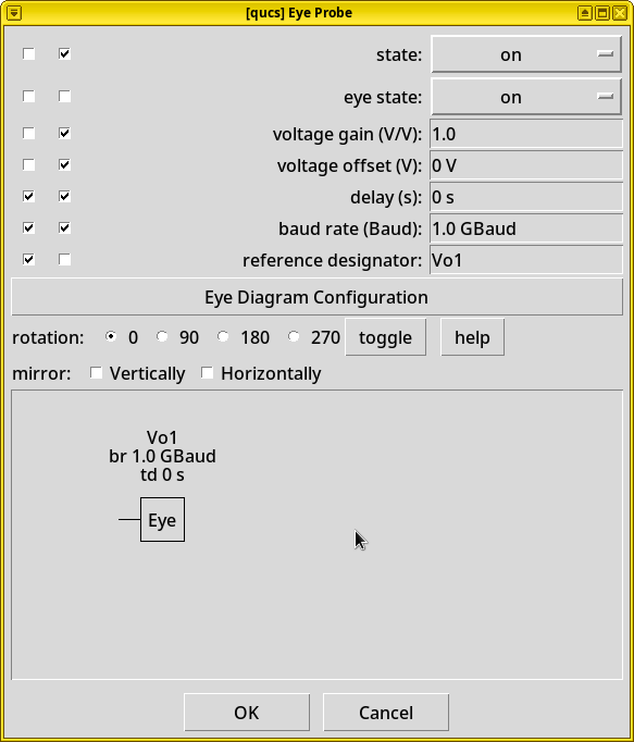
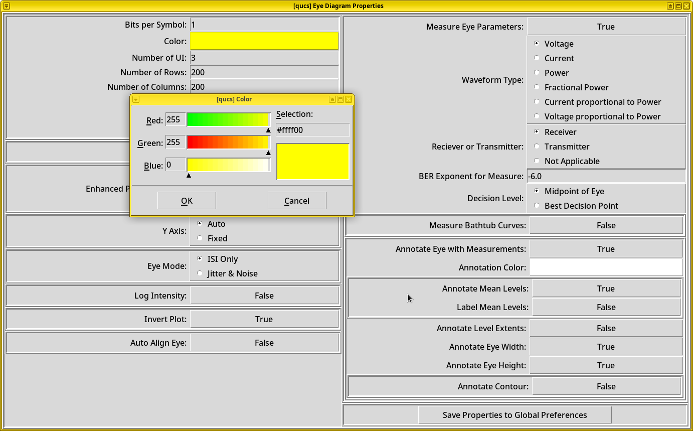
Add an eye probe. In the Add Part dialog, choose
. Click Eye
Diagram Configuration. Set Measure Eye Parameters to
True, and change the ::guilabel::Color to yellow (255, 255, 0)
to improve diagram readability. By default, the eye diagram is
black-and-white. Then close this window.
Tip
Press Enter to apply changed R, G, or B values. It’s not necessary to click Save Properties to Global Preferences, by default these options are already applied to a single schematic.
Place the probe and wire the circuit. Place the eye probe on the schematic. Wire the eye probe to DUT’s Port 2.
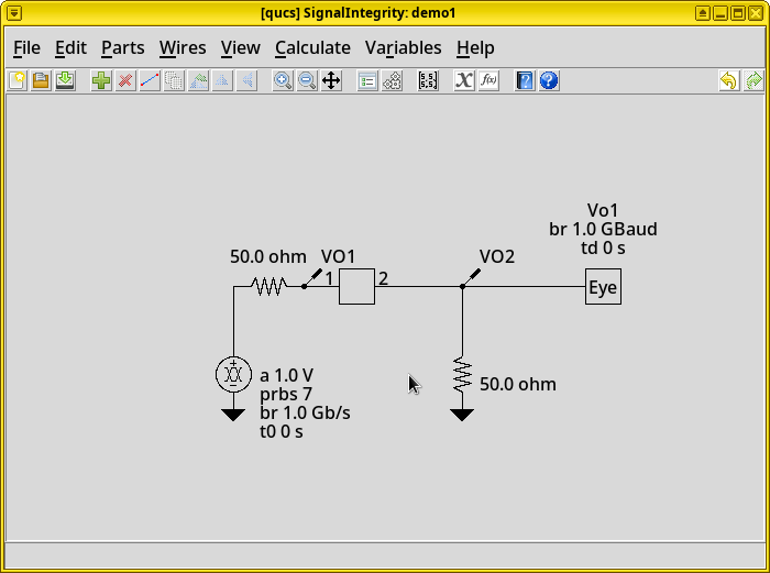
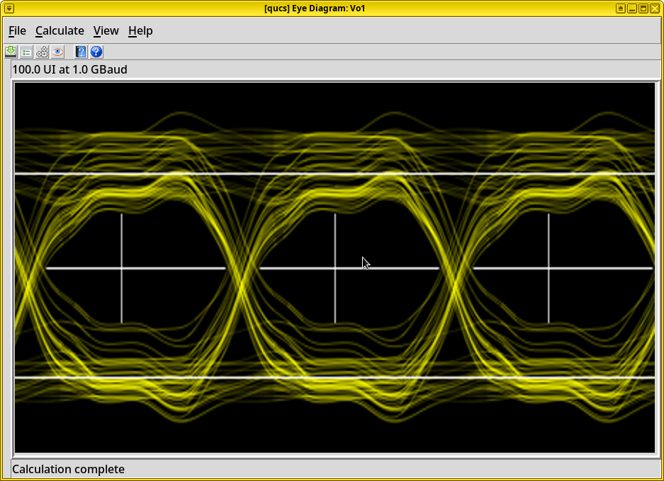
Run simulation. Click Calculate on the menu, choose Simulate. After simulation finishes, it opens two plots, an eye diagram plot and a time-domain line chart.
Results. The eye diagram clearly shows our parallel-plate waveguide has an extremely poor signal integrity. We will discuss the significance of this result at the end of this tutorial.
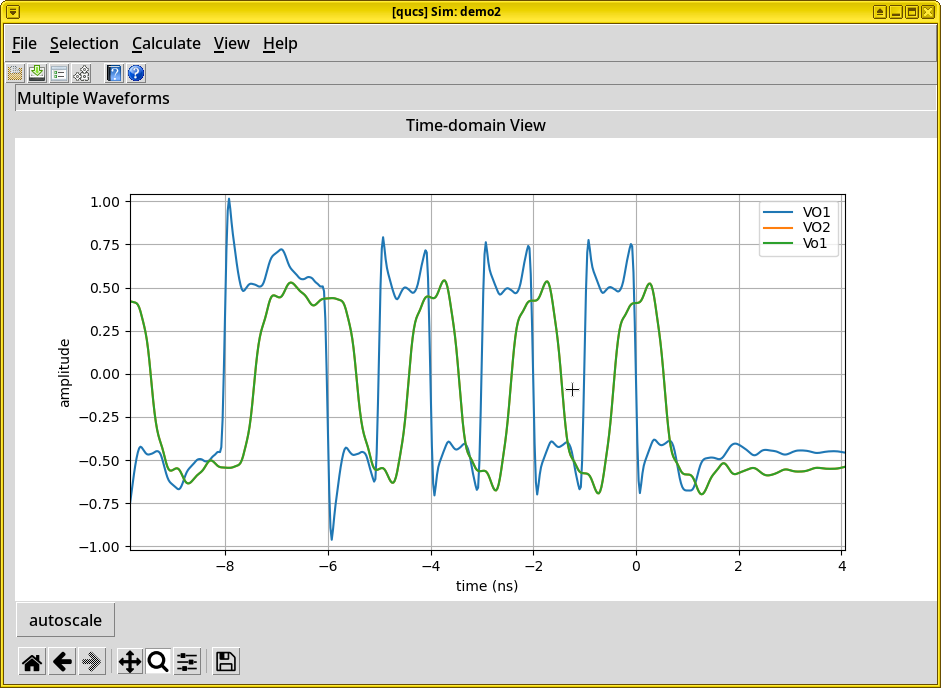
Zoom in. The time-domain line chart can be zoomed by pressing the “Magnifying Glass” button and drag a rectangle on a part of the waveform of interest. One can see that the overshoots, undershoots and rise-time degradation is similar to the previous impulse signal analysis.