Primitives

Primitives are the building blocks to create 1D, 2D, 3D shapes, so that one can create simple object such as a Curve, a Polygon, a Box, or a Sphere. More complex structures can be created by combining various primitives. For example, a metal sheet with cylindrical holes can be achieved by combining a metal box with several air cylinders.

Each shape created by a Primitive function is associated with a Property, representing its material or computational properties independent of its geometry. For example, by associating the same Box primitive to different properties, the same box can be a metal box, a plastic box, a glass box, or a virtual box for injecting or logging the electromagnetic field.

Relationship to Properties

A primitive is a geometrical shape, which is always derived from a physical or non-physical material known as a property. Together, they form physical and non-physical objects in the CSXCAD model. In principle, any properties can derive any primitives. For example, an excitation source is added to the model by creating a property via AddExcitation(), and deriving a Box primitive from it via AddBox().

Important

To create a meaningful object, remember to always create at least one property (such as a Metal) before creating any primitives.

Shapes

Box

The Box is the most simple primitive in CSXCAD. It is as well the most used primitive since it usually matches the given Cartesian or cylindrical FDTD mesh. Furthermore this primitive is the only one which shape depends on the chosen coordinate system it is defined with.

OctavePython

AddBox() function definition:

CSX = AddBox(CSX, 'propName', 1, start, stop, varargin);

• CSX: The original CSX structure.

• propName: Name of the assigned property.

• prio: Priority of the primitive, see Priority.

• start: [x y z] First (start) coordinate.

• stop: [x y z] Second (stop) coordinate.

• varargin: A key/value list of primitives variable arguments.

  • CoordSystem: See Coordinate Systems.

  • Transform, {array}: See Transformation.

Examples

1. Create a Cartesian box from x=[-100 to +100], y=[-50 to 0] and z=[-50 to 10]:

   OctavePython

   % create properties AddConductingSheet(), AddMaterial(), etc.
   csx = AddMetal(csx, 'metal'); % create PEC with propName 'metal'
   csx = AddBox(csx, 'metal', 1, [-100 -50 -50], [100 0 10]);
   

   

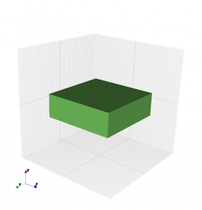
   Certesian Box example.

2. In case of a cylindrical system, create a cylindrical box from r=[50 to 70], alpha=[pi/2 to 3*pi/2] and z=[-50 to 10]:

   OctavePython

   % create properties AddConductingSheet(), AddMaterial(), etc.
   csx = AddMetal(csx, 'metal'); % create PEC with propName 'metal'
   csx = AddBox(csx, 'metal', 1, [50 pi/2 -50], [70 3*pi/2 10]);
   

   Note

   Although AddCylindricalShell() may appear to be the appropriate function to define a cylinder when using a cylindrical coordinate system, AddBox() is actually better suited because the structure will be meshed correctly. If AddCylindricalShell() is used, it is possible that the meshed cylinder will not be meshed correctly, as shown in the example below.

3. In case of a Cartesian FDTD setup, define a cylindrically shaped box from r=[50 to 70], alpha=[pi/2 to 3*pi/2] and z=[-50 to 10]:

   OctavePython

   % create properties AddConductingSheet(), AddMaterial(), etc.
   csx = AddMetal(csx, 'metal'); % create PEC with propName 'metal'
   
   % use 'CoordSystem' to enable Cylindrical coordinates even in a
   % Cartesian mesh.
   csx = AddBox(csx, 'metal', 1, [50 pi/2 -50], [70 3*pi/2 10], 'CoordSystem', 1);
   

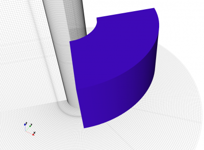
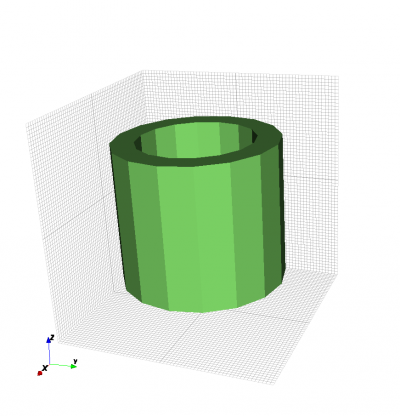
   Left: Cylindrical Box example. Right: Comparison of cylinders defined via AddCylindricalShell() (outer) and AddBox() (inner)

Sphere

The sphere primitive is defined by its central point and radius.

OctavePython

AddSphere() function definition:

CSX = AddSphere(CSX, propName, prio, center, rad, varargin)

• CSX: The original CSX structure.

• propName: Name of the assigned property.

• prio: Priority of the primitive, see Priority.

• center: Coordinate of the center point of the sphere.

• rad: Radius of the sphere.

• varargin: A key/value list of primitives variable arguments.

  • CoordSystem: See Coordinate Systems.

  • Transform, {array}: See Transformation.

Example

1. Create a sphere at (0, 0, 0) with radius 200:

   OctavePython

   % create properties AddConductingSheet(), AddMaterial(), etc.
   csx = AddMetal(csx, 'metal'); % create PEC with propName 'metal'
   csx = AddSphere(csx, 'material', 1, [0 0 0], 200);
   

   

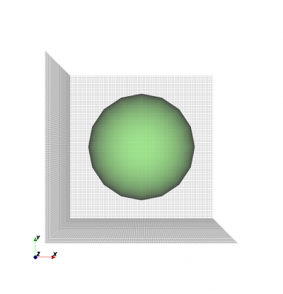
   Sphere example.

Spherical Shell

The spherical shell primitive is defined by its central point, radius and shell thickness.

OctavePython

AddSphericalShell() function definition:

CSX = AddSphericalShell(CSX, propName, prio, center, rad, shell_width, varargin)

• CSX: The original CSX structure.

• propName: Name of the assigned property.

• prio: Priority of the primitive, see Priority.

• center: Coordinate of the center point of the sphere.

• rad: Radius of the spherical shell.

• shell_width: Thickness of the shell.

  • The inner radius of this shell is rad - shell_width / 2.

  • The outer radius of this shell is rad + shell_width / 2.

• varargin: A key/value list of primitives variable arguments

  • CoordSystem: See Coordinate Systems.

  • Transform, {array}: See Transformation.

Example

1. Create a hollow metal sphere at (0, 0, 0) with radius 50 and thickness 10:

   OctavePython

   % create properties AddConductingSheet(), AddMaterial(), etc.
   csx = AddMetal(csx, 'metal'); % create PEC with propName 'metal'
   csx = AddSphericalShell(csx, 'metal', 10, [0 0 0], 50, 10);
   

   

   Spherical shell example.

Cylinder

A cylindrical primitive is defined by its midpoints of the first and last faces, and the radius of the cylinder. The axis of the cylinder will be along the start - stop points with the two cylinder faces being perpendicular to this axis.

Note

If the mesh already uses the Cylindrical coordinate system, use AddBox() instead.

OctavePython

AddCylinder() function definition:

CSX = AddCylinder(CSX, propName, prio, start, stop, rad, varargin)

• CSX: The original CSX structure

• propName: Name of the assigned material

• prio: Priority of the primitive, see Priority.

• start: [x y z] start point of the cylinder (midpoint of the first cylinder face).

• stop: [x y z] stop point of the cylinder (midpoint of the second cylinder face).

• rad: Radius of the cylinder.

• varargin: A key/value list of primitives variable arguments.

  • CoordSystem: See Coordinate Systems.

  • Transform, {array}: See Transformation.

Example

1. Create a metal cylinder from (0, 0, -300) to (0, 200, 300) with radius 300:

   OctavePython

   % create properties AddConductingSheet(), AddMaterial(), etc.
   csx = AddMetal(csx, 'metal'); % create PEC with propName 'metal'
   csx = AddCylinder(csx, 'metal', 1, [0 0 -300], [0 200 300], 300);
   

   

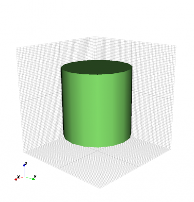
   Cylinder example.

Cylindrical Shell

A cylindrical shell primitive is defined by its midpoints of the first and last faces, the radius of the cylinder, and shell thickness.

Note

If the mesh already uses the Cylindrical coordinate system, use AddBox() instead.

OctavePython

AddCylindricalShell() function definition:

CSX = AddCylindricalShell(CSX, propName, prio, start, stop, rad, shell_width, varargin)

• CSX: default first argument, containing the CSXCAD data structure.

• propName: name of the (previously defined) property (e.g. a metal or material).

• start, stop: [x y z] coordinates of the start and end points of the cylinder central axis.

• rad: radius of the cylinder.

• shell_width: width of the cylinder shell.

  • The inner radius of this shell is rad - shell_width / 2.

  • The outer radius of this shell is rad + shell_width / 2.

• varargin: a key/value list of primitives variable arguments.

  • CoordSystem: See Coordinate Systems.

  • Transform, {array}: See Transformation.

Example

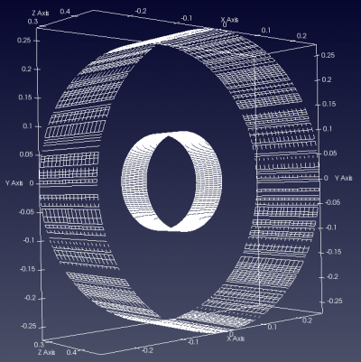
1. Create a cylindrical shell with radius 30 drawing unit and shell thickness of 5 drawing unit, made of plexiglass:

   OctavePython

   % create properties AddConductingSheet(), AddMaterial(), etc.
   csx = AddMaterial(csx, 'plexiglass');
   csx = SetMaterialProperty(csx, 'plexiglass', 'Epsilon', 2.22);
   start = [0 0 -40];
   stop  = [0 0  40];
   csx = AddCylindricalShell(csx, 'plexiglass', 5, start, stop, 30, 5);
   

   

   Cylindrical shell example.

Curve

A 1D curve is defined by its coordinate arrays.

OctavePython

AddCurve() function definition:

CSX = AddCurve(CSX, propName, prio, points, varargin)

• CSX: The original CSX structure.

• propName: Name of the assigned property.

• prio: Priority of the primitive, see Priority.

• points: Two-dimensional coordinates of the base polygon. Array column refers to point number, array row refers to its x, y, z positions.

  • points(1, point_number): position x of point_number.

  • points(2, point_number): position y of point_number.

  • points(3, point_number): position z of point_number.

• varargin: A key/value list of primitives variable arguments.

  • CoordSystem: See Coordinate Systems.

  • Transform, {array}: See Transformation.

Example

1. This example creates a Biquad antenna from thin metal on y=0, with length of each side= \(\sqrt{50}\):

   OctavePython

   points(1, 1) =  0; points(2, 1) = 0; points(3, 1) = 0;
   points(1, 2) =  5; points(2, 2) = 0; points(3, 2) = 5;
   points(1, 3) = 10; points(2, 3) = 0; points(3, 3) = 0.5;
   points(1, 4) = 15; points(2, 4) = 0; points(3, 4) = 5;
   points(1, 5) = 20; points(2, 5) = 0; points(3, 5) = 0;
   points(1, 6) = 15; points(2, 6) = 0; points(3, 6) = -5;
   points(1, 7) = 10; points(2, 7) = 0; points(3, 7) = -0.1;
   points(1, 8) =  5; points(2, 8) = 0; points(3, 8) = -5;
   points(1, 9) =  0; points(2, 9) = 0; points(3, 9) = 0;
   
   % create properties AddConductingSheet(), AddMaterial(), etc.
   csx = AddMetal(csx, 'metal');
   csx = AddCurve(csx, 'metal', 10, points);
   

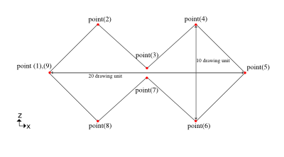
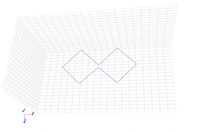
   Left: Biquad with points annotated. Right: Biquad model.

Wire

Define a cylinder-like wire by its coordinate arrays and radius.

OctavePython

AddWire() function definition:

CSX = AddWire(CSX, propName, prio, points, wire_rad, varargin)

• CSX: The original CSX structure

• propName: Name of the assigned property.

• prio: Priority of the primitive, see Priority.

• points: Two-dimensional coordinates of the base polygon. Array column refers to point number, array row refers to its x, y, z positions.

  • points(1, point_number): position x of point_number.

  • points(2, point_number): position y of point_number.

  • points(3, point_number): position z of point_number.

• wire_rad: Wire radius.

• varargin: A key/value list of primitives variable arguments.

  • CoordSystem: See Coordinate Systems.

  • Transform, {array}: See Transformation.

Example

1. This example creates a Biquad antenna from wire of radius 0.1 on xz-plane, with length of each side=:math:sqrt{50}:

OctavePython

points(1, 1) =  0; points(2, 1) = 0; points(3, 1) = 0;
points(1, 2) =  5; points(2, 2) = 0; points(3, 2) = 5;
points(1, 3) = 10; points(2, 3) = 0; points(3, 3) = 0.5;
points(1, 4) = 15; points(2, 4) = 0; points(3, 4) = 5;
points(1, 5) = 20; points(2, 5) = 0; points(3, 5) = 0;
points(1, 6) = 15; points(2, 6) = 0; points(3, 6) = -5;
points(1, 7) = 10; points(2, 7) = 0; points(3, 7) = -0.1;
points(1, 8) =  5; points(2, 8) = 0; points(3, 8) = -5;
points(1, 9) =  0; points(2, 9) = 0; points(3, 9) = 0;

% create properties AddConductingSheet(), AddMaterial(), etc.
csx = AddMetal(csx, 'metal');
csx = AddWire(csx, 'metal', 10, points, 0.1);

Polygon

A polygon is defined by its two dimensional shape in form of a polygon, its normal direction and elevation.

OctavePython

AddPolygon() function definition:

CSX = AddPolygon(CSX, propName, prio, normDir, elevation, points, varargin)

• CSX: The original CSX structure.

• propName: Name of the assigned property.

• prio: Priority of the primitive, see Priority.

• normDir: The normal direction of the polygon (0->x, 1->y, 2->z).

• points: Two-dimensional coordinates p(i,j) of the base polygon.

• elevation: Elevation in normal direction.

• varargin: A key/value list of primitives variable arguments.

  • CoordSystem: See Coordinate Systems.

  • Transform, {array}: See Transformation.

Note

1. The polygon has to be defined using Cartesian coordinates. For use with cylindrical mesh, set CoordSystem to 0 (Matlab/Octave) or call SetCoordinateSystem() to force Cartesian coordinates.

2. Each column j represents a vertex in the points matrix. The number of columns equals the number of points.

3. Each row represents projection of the point on the axis in the order of right hand rule. For example: if object is normal to y axis (normDir = 1), the first and second row contain z and x coordinates respectively. The number of rows is two.

Example

1. A star shaped polygon located in normal direction at z = 0:

   OctavePython

   p(1, 1) = -100; p(2, 1) = -100;
   p(1, 2) =    0; p(2, 2) =  -50;
   p(1, 3) =  100; p(2, 3) = -100;
   p(1, 4) =   50; p(2, 4) =    0;
   p(1, 5) =  100; p(2, 5) =  100;
   p(1, 6) =    0; p(2, 6) =   50;
   p(1, 7) = -100; p(2, 7) =  100;
   p(1, 8) =  -50; p(2, 8) =    0;
   
   % >> p
   % p =
   %
   %   -100     0   100    50   100     0  -100   -50
   %   -100   -50  -100     0   100    50   100     0
   
   % create properties AddConductingSheet(), AddMaterial(), etc.
   csx = AddMetal(csx, 'metal');
   
   % If the mesh coordinate is cylindrical, this primitive must still be
   % in Cartesian coordinate. 'CoordSystem' optional if the mesh is Cartesian.
   csx = AddPolygon(csx, 'metal', 1, 2, 0, p, 'CoordSystem', 0)
   

   

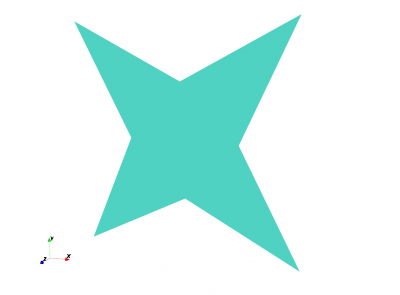
   Polygon example.

Extruded Polygon

An extruded polygon is defined by its two dimensional base shape in form of a polygon, its normal direction, elevation and thickness.

Note

The polygon has to be defined using Cartesian coordinates. For use with cylindrical mesh, set CoordSystem to 0.

OctavePython

AddLinPoly() function definition:

CSX = AddLinPoly(CSX, propName, prio, normDir, elevation, points, Length, varargin)

• CSX: The original CSX structure.

• propName: Name of the assigned property.

• prio: Priority of the primitive, see Priority.

• normDir: The normal direction of the polygon (0->x, 1->y, 2->z).

• points: Two-dimensional coordinates of the base polygon; see above.

• elevation: Elevation in normal direction.

• length: Linear extrusion in normal direction, starting at elevation.

• varargin: See primitives variable arguments.

  • CoordSystem: See Coordinate Systems.

  • Transform, {array}: See Transformation.

Important

The polygon has to be defined using Cartesian coordinates. For use with cylindrical mesh, set CoordSystem to 0.

Example

1. A star shaped polygon extruded in z direction:

   OctavePython

   p(1, 1) = -100; p(2, 1) = -100;
   p(1, 2) = 0;    p(2, 2) = -50;
   p(1, 3) = 100;  p(2, 3) = -100;
   p(1, 4) = 50;   p(2, 4) = 0;
   p(1, 5) = 100;  p(2, 5) = 100;
   p(1, 6) = 0;    p(2, 6) = 50;
   p(1, 7) = -100; p(2, 7) = 100;
   p(1, 8) = -50;  p(2, 8) = 0;
   
   % create properties AddConductingSheet(), AddMaterial(), etc.
   csx = AddMetal(csx, 'metal')
   
   % If the mesh coordinate is cylindrical, this primitive must still be
   % in Cartesian coordinate. 'CoordSystem' optional if the mesh is Cartesian.
   csx = AddLinPoly(csx, 'metal', 1, 2, 2, p, 100, 'CoordSystem', 0)
   

   

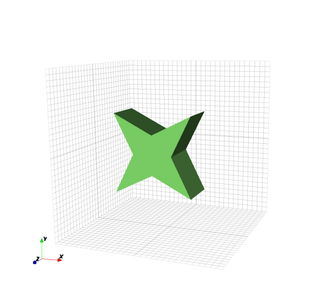
   LinPoly example.

Rotational Polygon

An rotational polygon is defined by its two dimensional base shape in form of a polygon, its normal direction, rotational axis and angle of rotation.

OctavePython

AddRotPoly() function definition:

CSX = AddRotPoly(CSX, materialname, prio, normDir, points, RotAxisDir, angle, varargin)

• CSX: The original CSX structure.

• materialname: Name of the assigned material property, created by :func:AddMetal` or :func:``AddMaterial.

• prio: Priority of the primitive, see Priority.

• normDir: The normal direction of the polygon e.g. x, y or z, or numeric (0->x, 1->y, 2->z).

• RotAxisDir: Rotational axis direction e.g. x, y or z, or numeric (0->x, 1->y, 2->z). * Note` it should be different to normal direction.

• points: Two-dimensional coordinates of the base polygon; see above

• angle: Rotation angle, optional, default is [0 2*pi] (e.g. [0 2*pi] for a full rotation).

• varargin: See primitives variable arguments.

  • CoordSystem: See Coordinate Systems.

  • Transform, {array}: See Transformation.

Important

The polygon has to be defined using Cartesian coordinates. For use with cylindrical mesh, set CoordSystem to 0.

Example

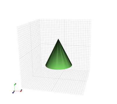
Left: Rotational Polygon example. Right: Cone example.

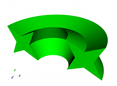
1. The same star shaped polygon, shifted in x-direction and rotated around the x-axis:

   OctavePython

   p(1, 1) = -100; p(2, 1) = -100;
   p(1, 2) =    0; p(2, 2) = -50;
   p(1, 3) =  100; p(2, 3) = -100;
   p(1, 4) =   50; p(2, 4) =    0;
   p(1, 5) =  100; p(2, 5) =  100;
   p(1, 6) =    0; p(2, 6) =   50;
   p(1, 7) = -100; p(2, 7) =  100;
   p(1, 8) =  -50; p(2, 8) =    0;
   
   p(1,:) = p(1,:) + 200; % shift in x-direction by 200
   
   % create properties AddConductingSheet(), AddMaterial(), etc.
   csx = AddMetal(csx, 'metal')
   
   % If the mesh coordinate is cylindrical, this primitive must still be
   % in Cartesian coordinate. 'CoordSystem' optional if the mesh is Cartesian.
   csx = AddRotPoly(csx, 'metal', 1, 2, p, 1, [0 pi], 'CoordSystem', 0)
   

2. A conical solid can be created by rotating a triangular polygon:

   OctavePython

   p(1, 1) =   0;  p(2, 1) = -100;
   p(1, 2) = 100;  p(2, 2) = -100;
   p(1, 3) =   0;  p(2, 3) =  100;
   
   % create properties AddConductingSheet(), AddMaterial(), etc.
   csx = AddMetal(csx, 'metal')
   csx = AddRotPoly(csx, 'metal', 1, 2, p, [1 0 0], [0, 2*pi])
   

Polyhedron

A polyhedron is the most general 3D primitive available for openEMS. It can be used to create a body with (nearly) any shape by defining a closed surface using verteces and faces.

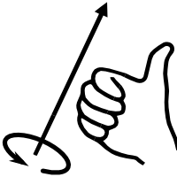
Verteces and Faces

Left: Tetrahedron, the simplest polyhedron. Right: The right hand rule. When using the right hand the thumb indicates the normal direction of the face and the fingers show the direction how to order the vertices for each face.

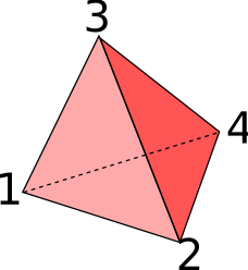
A polyhedron is the most general shape that can be defined in openEMS. Polyhedrons are defined by their vertices and faces. In openEMS each vertex is an array containing the x, y and z coordinates of the point. All faces must contain the vertices in a right-handed order with the normal direction for each face pointing out of the solid. In the example of the tetrahedron the four faces would be {1, 2, 3}, {2, 4, 3} and {1, 3, 4}.

Note

• The polyhedron must be a closed surface for 3D discretisation

• All faces must contain the vertices in a right-handed order with the normal direction for each face pointing out of the solid

OctavePython

AddPolyhedron() function definition:

CSX = AddPolyhedron(CSX, propName, prio, vertices, faces, varargin)

• CSX: The original CSX structure.

• propName: Name of the assigned property.

• prio: Priority of the primitive, see Priority.

• vertices: Cell array of all vertices.

• faces: Cell array of all faces.

• varargin: A key/value list of primitives variable arguments.

  • CoordSystem: See Coordinate Systems.

  • Transform, {array}: See Transformation.

Example

OctavePython

% example tetrahedron
vertices{1} = [0 0 0];
vertices{2} = [1 0 0];
vertices{3} = [0 1 0];
vertices{4} = [0 0 1];
faces{1} = [0 2 1];
faces{2} = [0 1 3];
faces{3} = [0 3 2];
faces{4} = [1 2 3];

% create properties AddConductingSheet(), AddMaterial(), etc.
csx = AddMetal(csx, 'metal');
csx = AddPolyhedron(csx, 'metal', 0, vertices, faces);

Coordinate Systems

The coordinates used to define a primitive are always assumed to be given in the coordinate system used globally (i.e. by the mesh’s coordinate system). In certain situations, it may be useful though to define a primitive in a coordinate system specifically for this single primitive.

In Matlab/Octave, the keyword for that is CoordSystem: 0 for Cartesian and 1 for a cylindrical coordinate system. In Python, use CSPrimitives’s SetCoordinateSystem() method.

Example

Define a box forcing a cylindrical coordinate representation:

OctavePython

% create properties AddConductingSheet(), AddMaterial(), etc.
csx = AddMetal(csx, 'metal');
csx = AddBox(csx, 'metal', 1, [50 pi/2 10], [70 3*pi/2 -50], 'CoordSystem', 1);

Transformation

All primitives can be translated, scaled and rotated with the Transform option. This option is added to the command which creates a primitive (AddBox, AddSphere, etc.). For example, in Matlab/Octave:

'Transform', {'Scale', '1, 1, 2', 'Rotate_X', pi / 4, 'Translate', '0, 0, 100'}

The transformations are applied in the order as given inside the {} brackets. That means, {'Scale', '1, 1, 2', 'Rotate_X', pi / 4} and {'Rotate_X', 'Scale', '1, 1, 2'} will lead to different results.

OctavePython

• {'Scale', 's'}:

  • Scale the primitive in x, y and z-direction equally by the factors s.

• {'Scale', 's_x, s_y, s_z'}:

  • Scale the primitive in x, y and z-direction by the factors s_x, s_y, s_z.

• {'Rotate_Origin', [ax, ay, az, angle]}:

  • Rotate the primitive by the given angle (in radians) around the given axis [0, 0, 0] --> [ax, ay, az].

• {'Rotate_X', angle}:

  • Rotate the primitive by the given angle (in radians). Rotations around the y and z axis are done accordingly with ‘Rotate_Y’ and ‘Rotate_Z’

• {'Translate', 't_x, t_y, t_z'}:

  • Translate the structure by the vector (t_x, t_y, t_z)

• {'Matrix', [4x4 matrix]}:

  • General affine transformation given as a 4 by 4 matrix. A 1 is appended internally to the row vector of the primtive nodes, so it becomes a four-dimensional row vector. A 0 is appended to edge vectors (directions). This row vector multiplied by the transform matrix gives the new coodinates. The first three rows/columns of the matrix are rotation/shear/scaling. The last column is [0; 0; 0; 1]. The last row is [shift_x, shift_y, shift_z, 1].

These transformations can be used to create for example an ellipsoid primitive.

Example

1. Add a translation and 30° rotation around the z-axis:

   OctavePython

   % TODO
   

2. Add a rotation around the axis=[1, 1, 0] by pi / 3 (30°):

   OctavePython

   % TODO
   

Warning

matlab documentation TBD.

Priority

An important concept in openEMS are the priorities assigned to each primitive. In regions where two or more primitives overlap, openEMS needs to decide which material property to assign to these regions. Here the priorities of the overlapping primitives become important: At each point openEMS will assign the material of the primitive with the highest priority. This way one can for example carve holes in a block of solid material by adding air primitives which have a higher priority. The diagrams below show how priorities will effect the material distribution for the simulations. If two blocks are overlapping, the one with the higher priority value will be chosen.

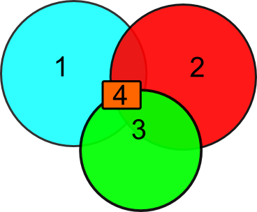
At points where two or more primitives overlap, the properties of the primitive with the highest priority value will be assigned.

For the more complicated case, where three or more blocks overlap, openEMS uses the block with the highest priority at each point. This way it is possible to create complicated shapes from the basic primitives by simply using primitives assigned to different materials and assign the priorities appropriately.

Exceptions:

• Non-physical properties, such as dump boxes, probe boxes, etc. are not affected by the priority system.

• Excitation Sources are not affected as well, since multiple (superpositioned) excitations are possible.

• The curve primitive as a 1D line element is not affected.

• Lumped elements are not affected.

Example: Metal Sheet With Cylindrical Holes

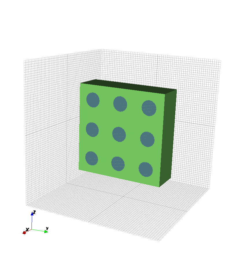
A holey metal sheet is easily created by combining a metal box and several air cylinders. Here it is important that the priority of the air cylinders is higher than the priority of the metal box. Only 3 steps are necessary to achieve this structure:

1. Define the materials for metal and air.

2. Add a metal box with AddBox(), set the priority to 1 (lowest priority).

3. Add air cylinders with coordinates that they are completely going through the metal sheet, set the priority to 2 (higher than 1).

The Matlab/Octave code for a metal sheet with 3x3 holes will be:

% Define a material with propName 'air'. Actually a vacuum, but the
% material property differences between air and vacuum is minimum.
csx = AddMaterial(csx, 'Air');
csx = SetMaterialProperty(csx, 'Air', 'Epsilon', 1, 'Mue', 1);

% create PEC with propName 'metal'
csx = AddMetal(csx, 'metal');

% define structure
csx = AddBox(csx, 'metal', 1, [-100 -300 -300], [100 300 300]);
for y=-1:1
    for z=-1:1
        csx = AddCylinder(csx, 'Air', 2, [-100 y*200 z*200], [100 y*200 z*200], 50);
    end
end

Complex Examples

More complex structures can be created by combining various primitives with specific priorities and transformations.

Mickey

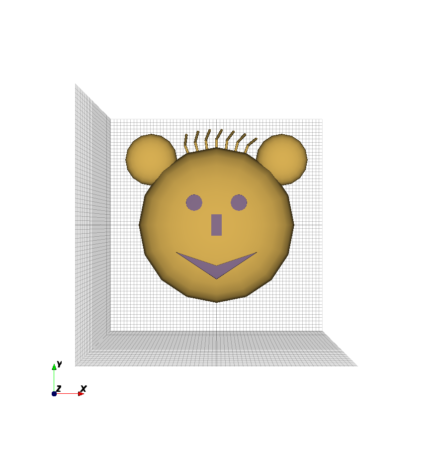
This structure was created by combining several scaled spheres, cylinders, and a polyhedron:

% materials
csx = AddMaterial(csx, 'Air');
csx = SetMaterialProperty(csx, 'Air', 'Epsilon', 1, 'Mue', 1);
csx = AddMetal(csx, 'metal'); %create PEC with propName 'metal'

% face
csx = AddSphere(csx, 'metal', 1, [0 0 0], 150, 'Transform', {'Scale', '2,2,1'});

% ears
csx = AddSphere( ...
    csx, 'metal', 1, ...
    [ sqrt(0.7 * 150 ^ 2) sqrt(0.7 * 150 ^ 2) 0], ...
    50, ...
    'Transform', {'Scale', '2,2,1'} ...
);
csx = AddSphere( ...
    csx, 'metal', 1, ...
    [-sqrt(0.7 * 150 ^ 2) sqrt(0.7 * 150 ^ 2) 0], ...
    50, ...
    'Transform', {'Scale', '2,2,1'} ...
);

%nose
csx = AddBox(csx, 'Air', 2, [-20 -40 -160], [20 40 160]);

% eyes
csx = AddCylinder(
    csx, 'Air', 2, ...
    [-sqrt(0.3 * 150 ^ 2) sqrt(0.3 * 150 ^ 2) -150], ...
    [-sqrt(0.3 * 150 ^ 2) sqrt(0.3 * 150 ^ 2) 150], ...
30);
csx = AddCylinder(
    csx, 'Air', 2, ...
    [ sqrt(0.3 * 150 ^ 2) sqrt(0.3 * 150 ^ 2) -150], ...
    [ sqrt(0.3 * 150 ^ 2) sqrt(0.3 * 150 ^ 2) 150], ...
30);

% hair
points = zeros(3,3);
points(:,1) = [0 290 0];
points(:,2) = [0 330 0];
points(:,3) = [20 360 50];
for i=-3:3
    csx = AddWire(csx, 'metal', 10, points, 5,' Transform', {'Rotate_Z', i * pi / 25});
end

% mouth
vertices{1} = [-150 -100 150];
vertices{2} = [0 -150 150];
vertices{3} = [150 -100 150];
vertices{4} = [0 -200 150];
vertices{5} = [-150 -100 -150];
vertices{6} = [0 -150 -150];
vertices{7} = [150 -100 -150];
vertices{8} = [0 -200 -150];

faces{1} = [1 2 3 0];
faces{2} = [4 7 3 0];
faces{3} = [4 5 1 0];
faces{4} = [6 7 3 2];
faces{5} = [1 5 6 2];
faces{6} = [7 6 5 4];

csx = AddPolyhedron(csx, 'Air', 0, vertices, faces);

Sphere Aggregation

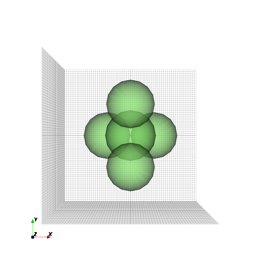
An aggregation of multiple spheres can easily be achieved. In this case there are 5 close packed spheres around the (0 0 0) point:

csx = AddMaterial(csx, 'Diel');
csx = SetMaterialProperty(csx, 'Diel', 'Epsilon', 5, 'Mue', 1);

rad = 150;
x = rad * tan(pi / 6);
y = rad / cos(pi / 6);
z = sqrt(x ^ 2 + y ^ 2);

coords=[ ...
    [-rad  0 -(x+y)/2]; ...
    [ rad  0 -(x+y)/2]; ...
    [   0  0  (x+y)/2]; ...
    [   0  z        0]; ...
    [   0 -z        0] ...
];

for i=1:length(coords(:,1)),
    csx = AddSphere(csx, 'Diel', 1, coords(i,:), rad);
end