S-Parameters Analysis via Qucs-S
Qucs is a free and open source circuit simulator for RF/microwave engineering, it’s capable of simulating circuits in both time and frequency domains.
Install
Qucs has a somewhat confusing development history, three different spinoffs exist.
Qucs. Development of the original Qucs started in the early 2000s, but was slowed down over time. Finally in ~2019, its underlying GUI framework Qt4 has been discontinued, making it uninstallable on most operating systems. Its Qucsator` engine has good RF simulation features, but limited time-domain capabilities with performance and convergence issues.
QucsStudio is a free-of-charge spinoff of Qucs with additional features, but it’s not free and open source software.
Qucs-S. The project Qucs-S is a fork of Qucs with a modernized codebase, aiming to support multiple SPICE backends for improved time-domain simulations, such as Ngspice. RF simulations still use the original Qucsator engine externally before Qucs-S 24.2.0 (meaning that an installation of the now-unavailable Qucs is still needed). After Qucs-S 24.2.0, Qucsator is now a builtin option.
Warning
For this tutorial, we use Qucs-S 25.1.0. Other Qucs spinoffs or older Qucs-S versions have features and user interface changes that are in conflict with this tutorial, so one should use Qucs-S 25.1.0 or newer when following this tutorial.
The Qucs-S packages in most operating systems are outdated, thus, Debian, Ubuntu, Fedora and openSUSE users should use the third-party maintained by Qucs-S projcet developers. It’s hosted on Open Build Service (OBS), installation instructions can be found in the following link.
Alternatively, if no package is available, a self-contained AppImage version is also available as a stop-gap measure before it’s packaged.
Download Qucs-S-25.1.0-linux-x86_64.AppImage, and grant it
execution permission:
chmod +x Qucs-S-25.1.0-linux-x86_64.AppImage
Enable Qucsator
As previously mentioned, Qucs-S uses Ngspice for simulation by default, but it lacks some features required for RF/microwave applications that we need. Hence, we must switch Qucs-S’s engine from Ngspice to Qucsator.
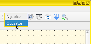
Switch the engine. Press the drop-down list at the top-right of the Qucs-S window. By default, it should show Ngspice, click it and change it to Qucsator.
Important
If the option Qucsator does not exist (it usually disappears when one quits and restarts the application), it means you’re affected by a bug in the AppImage version of Qucs-S. See qucsator_bug for the solution.
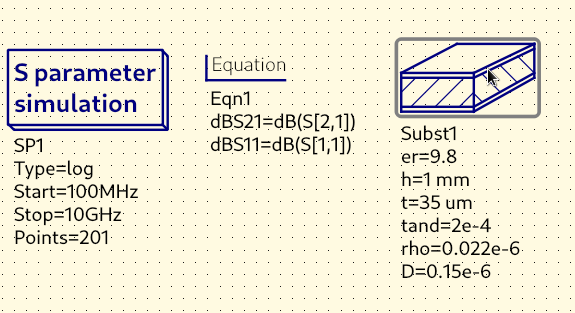
S-Parameter Simulation Skeleton
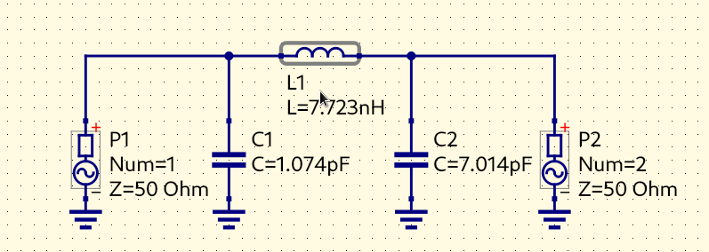
To perform frequency-domain analysis in Qucs (Qucs-S), we need to add several components in multiple steps: adding two power sources, entering two equations for calculating scalar S-parameters \(S_{11}\) and \(S_{21}\), adding an “S-parameter simulation” block with parameters, and inserting the DUT in the middle between the two ports.
Important
Before a filter is synthesized, Qucs-S must be switched to use Qucsator as its engine as described in Enable Qucsator. Otherwise a broken schematic would be synthesized with non-functional equations - S-parameter simulations won’t work correctly.
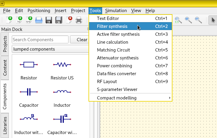
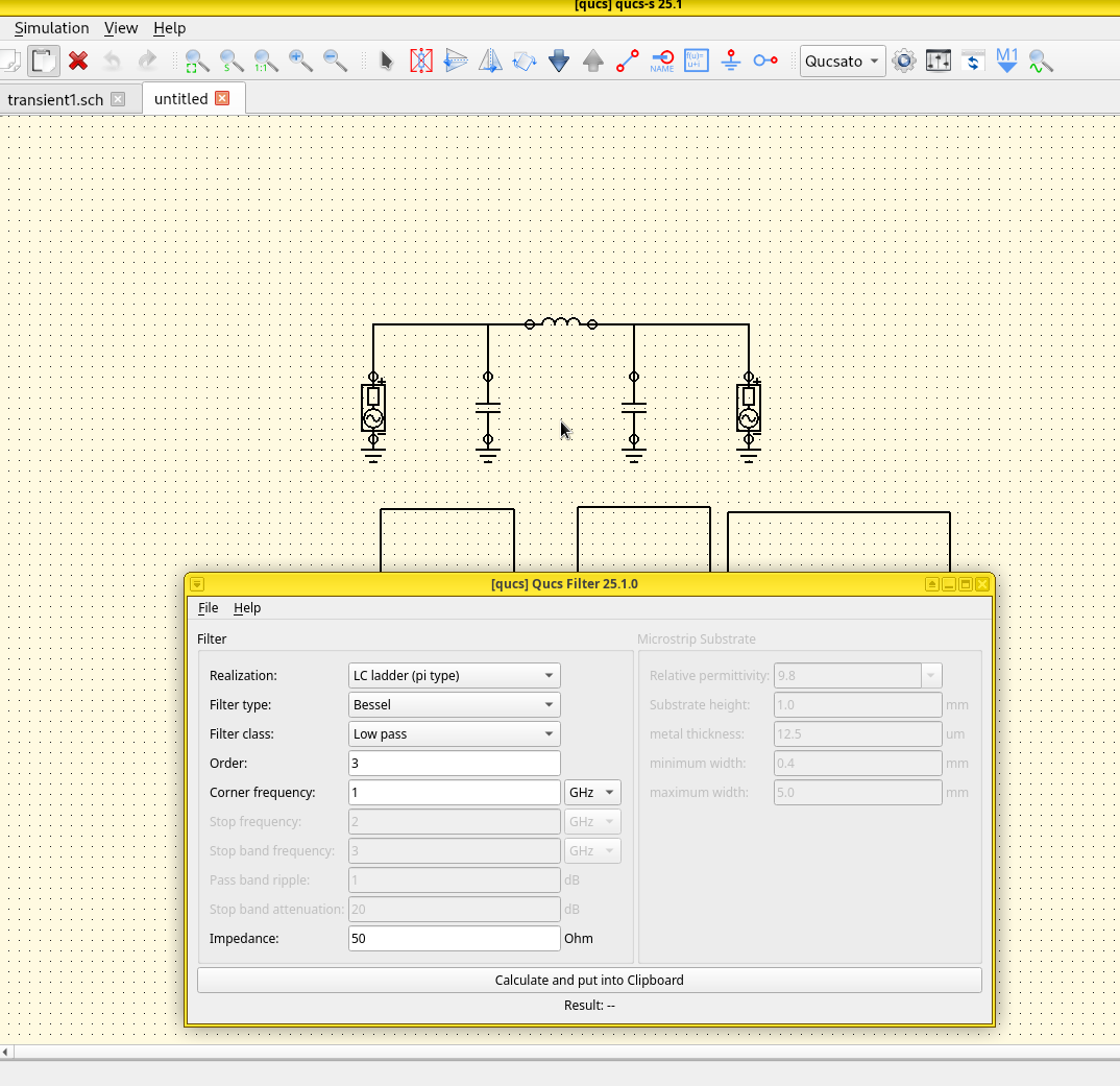
Open the filter wizard. A trick allows us to quickly setting up a skeleton - “borrowing” the setup generated by Qucs’s filter synthesis wizard. Click .
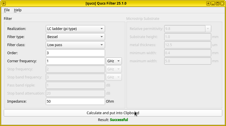
Synthesize a filter. In the opened dialog, generate the default low-pass LC filter by pressing Calculate and put into Clipboard, without changing any parameters.
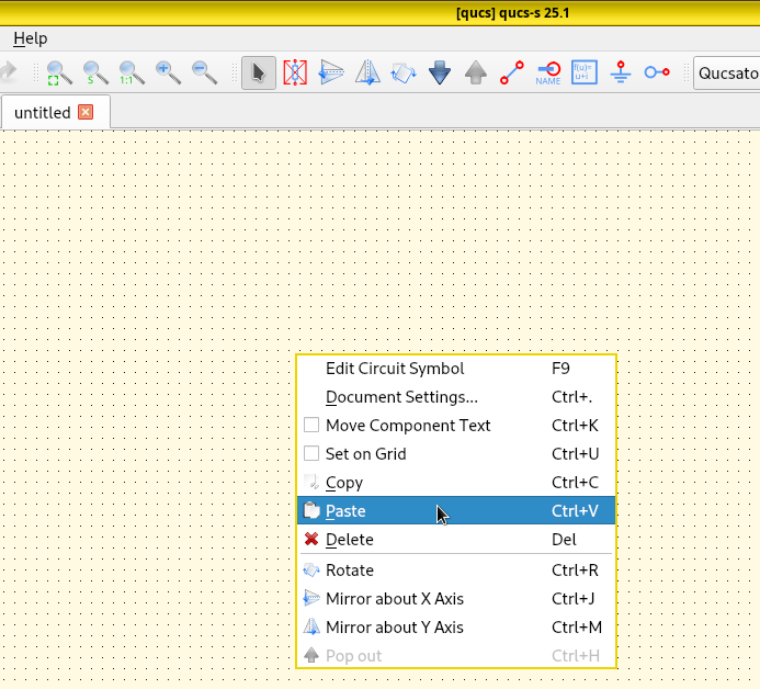
Paste it into schematic. Do not close the filter dialog yet. Now right-click the schematic, click Paste. Paste the synthesized filter circuit onto the page by left-clicking. After pasting, it’s free to close the filter dialog.
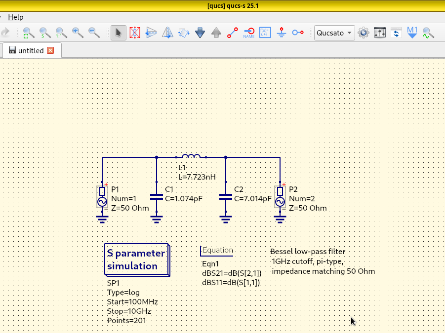
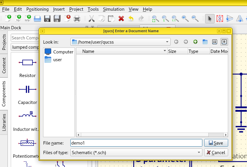
Save the schematic to disk. Press the 💾 (floppy disk) button, and choose a path. This is required before starting a simulation.
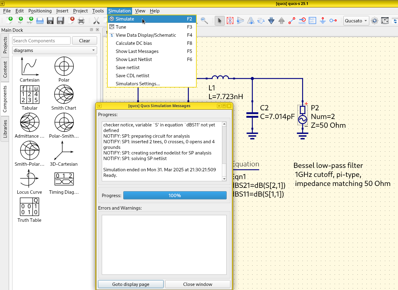
Run simulation. Select . A dialog should pop up without warnings or errors.
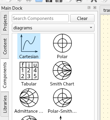
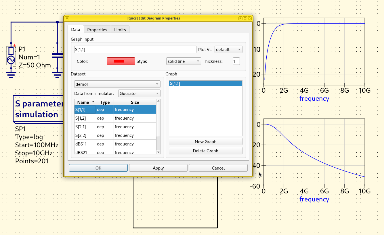
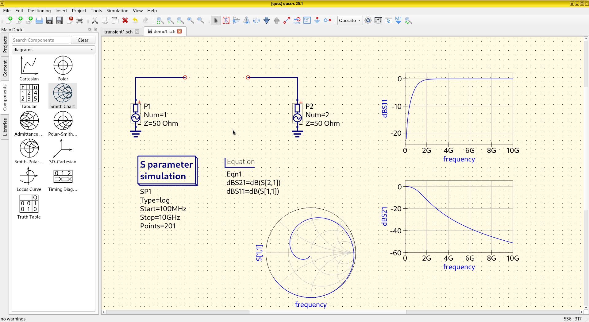
Add a Cartesian plot. On the Main Dock on the left, switch from lumped components to diagrams. Click the Cartesian component.
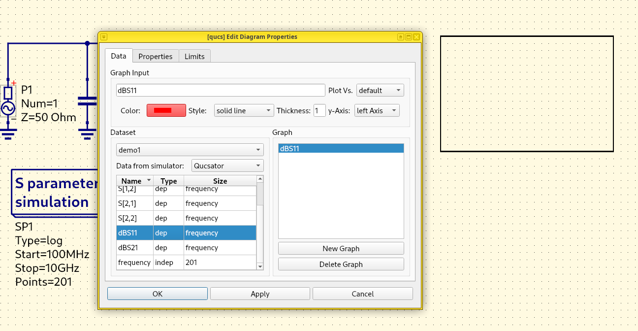
Plot dbS11. Click the schematic to place the component. In
the dialog, double-click the scalar dbS11 to add it into the
Graph item list, then press OK.
Important
The scalars dBS11 and dbS21 are not to be confused with the
complex S-parameters S[1,1] and S[2,1]. In particular, the
Smith chart won’t work with a scalar value.
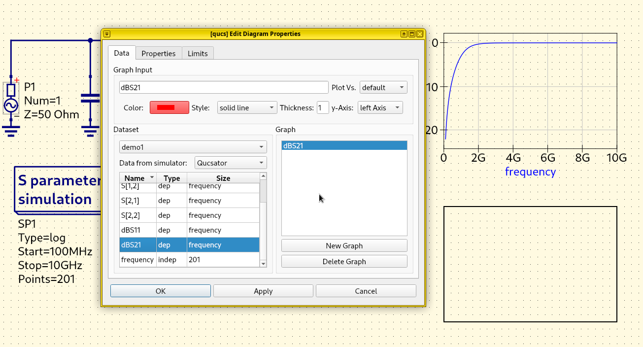
Plot dbS21. Repeat the same steps above, add another
Cartesian component to the schematic. Click the schematic to
place it. In the dialog, double-click the scalar dBS21 (not the
complex S[2,1]) to add this array into the Graph item
list. Click OK.
Add a Smith chart. Click the Smith Chart component on the Main Dock.
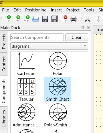
Plot S[1,1]. Click the schematic to place the component. In the
dialog, double-click S[1,1] (not dBS11) to add this array into the
Graph item list. Click “OK”.
Hint
All subsequent mouse clicks will keep adding components to the schematic. To stop, press Esc or click the Select button (cursor icon) on the menu bar.
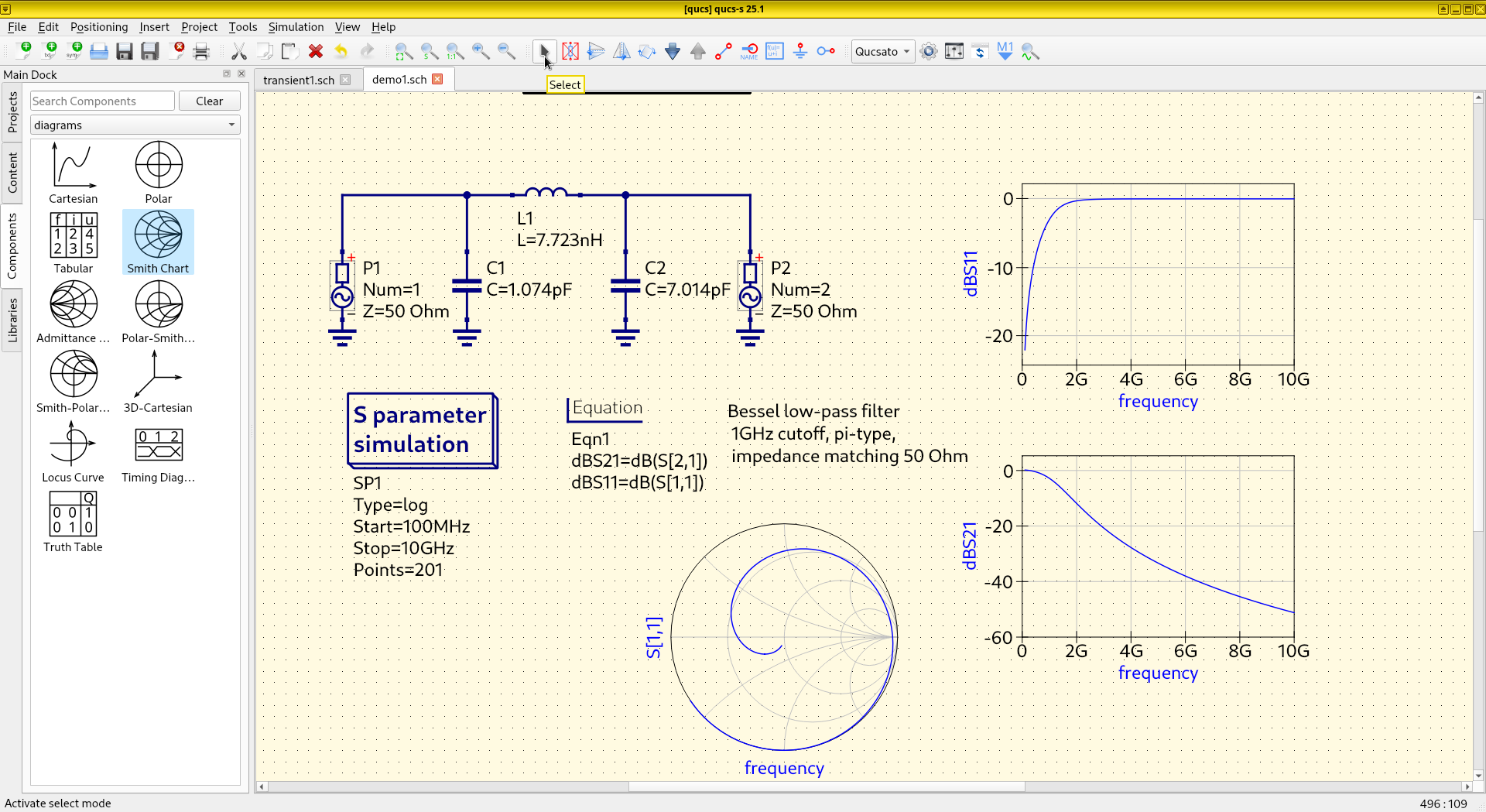
Plotting. Now we have a fully-functional S-parameter simulation skeleton with S-parameters on two line chart and a Smith chart.
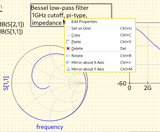
Delete the text label. The next step is to delete the filter, leaving only the simulation skeleton. First, select the text label Bessel low-pass filter 1 GHz cutoff, … by left-clicking it and pressing the Delete key on the keyboard (or by right-cilking it and pressing the Delete option). This text label would be useless and misleading if it’s left here.
Delete the inductor, capacitors, and wire segments. Select the inductor and delete it by pressing the Delete key on the keyboard. Delete the capacitors using the same procedure.
Hint
It’s difficult to delete a wire segment without highlighting the entire wire. If you have trouble selecting a segment, try dragging the mouse to highlight a rectangle that contains only that segment.
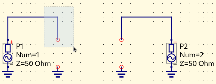
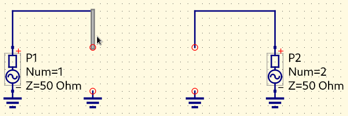
Clean Skeleton Obtained. After all useless components are wires have been deleted, the simulation skeleton is clean to use.
Two-Port S-Parameter Analysis
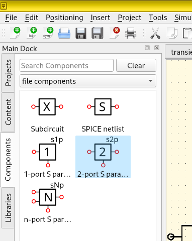
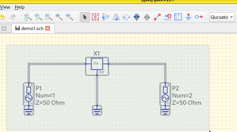
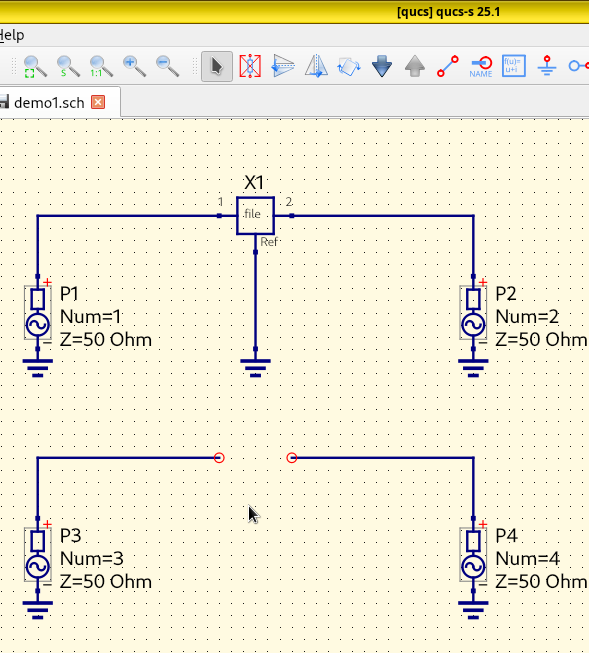
Add an S-parameter-defined component. On the left Main Dock, switch from diagram (or lumped components) to file components. Click 2-port S-parameters, place it on the schematic.
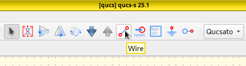
Wire component together. Click the Wire icon on the menu bar. Connect the DUT’s Port 1 to the left, connect Port 2 to the right, and wire the Reference Port downwards.
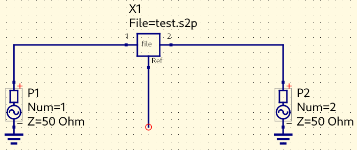
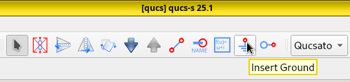
Add a ground. Click Ground Node on the menu bar, add a ground below wire to the reference port.
Hint
Don’t forget to press Esc to exit from insert mode, otherwise every mouse click results in more Ground Nodes on the schematic.
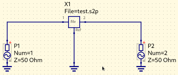
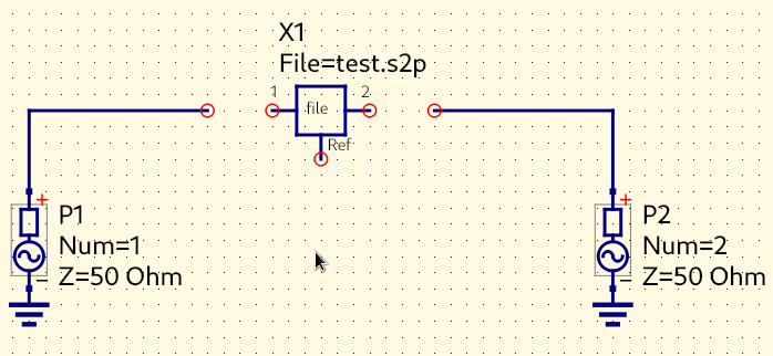
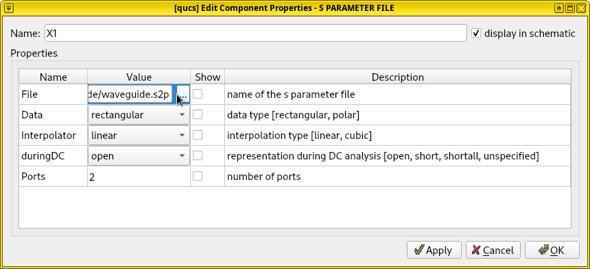
Set S-parameter path. Double click the file component X1. In the opened dialog, press the … button to change the path of the Touchstone file that backs this parameter-defined component. Pick the Touchstone file created by the openEMS simulation. Also, uncheck the Show option, since the file path is extremely long and visually cluttering. Press OK.
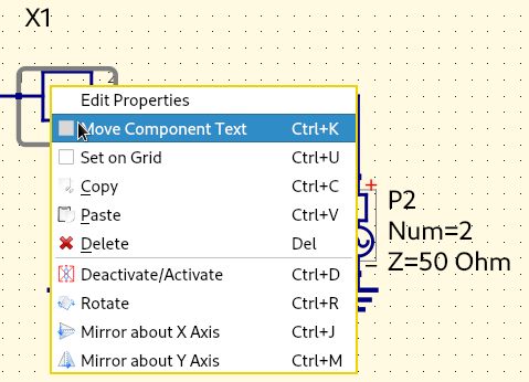
Move Component Text. One may also want to adjust the position of the text label X1 to be directly above the component box (since the space occupied by the file path has gone) to improve readability. This can be done by right-clicking the component, select Move Component Text, then drag the text to a new position.
Run simulation. Select Simulation and click Simulate. A dialog should pop up without warnings or errors.
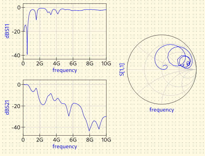
Results. Now the S-parameters from our simulation should appear on the Smith and line charts.
Comparison with Microstrip
In the analysis of RF/microwave devices, We often need to compare the behavior of different circuits. Using the microstrip as an example (as the limiting case of a parallel-plate waveguide when the lower plate has an infinite size), we perform a simple comparison here.
Select and move the existing circuit. Drag the mouse and select the entire circuit, move it upwards to free up some space. Press Control-C to copy this circuit, then press Control-V to paste a new instance and place it below the original.
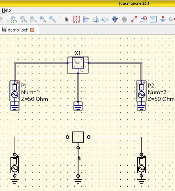
Delete the extra file-defined component. Delete X2 and its ground connect.
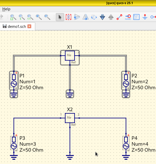
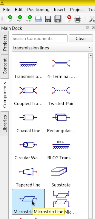
Add a microstrip. On the left Main Dock, switch to
transmission lines. Click Microstrip Line,
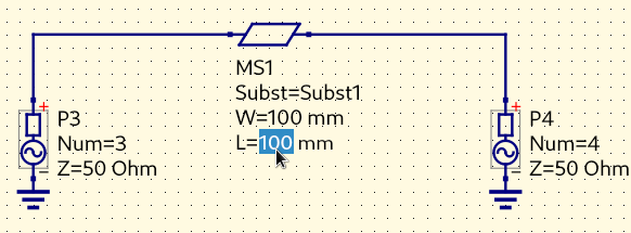
and place it between Port 3 and Port 4.
Change its W (width) and L to 100 mm. Apply the
numer change by pressing Enter.
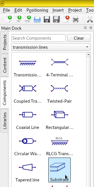
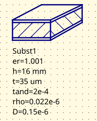
Add a substrate that supports the microstrip. On the left
Main Dock, click Substrate, and place it
at the bottom of the schematic. Change parameter er to 1.001
(don’t use 1.0, the Qucs-S’s internal formula is singular here).
Change parameter h (height) to 16 mm.
Add new equations for scalar S33 and S43. Double-click the Equation component.
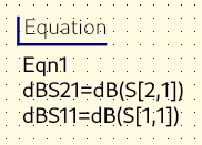
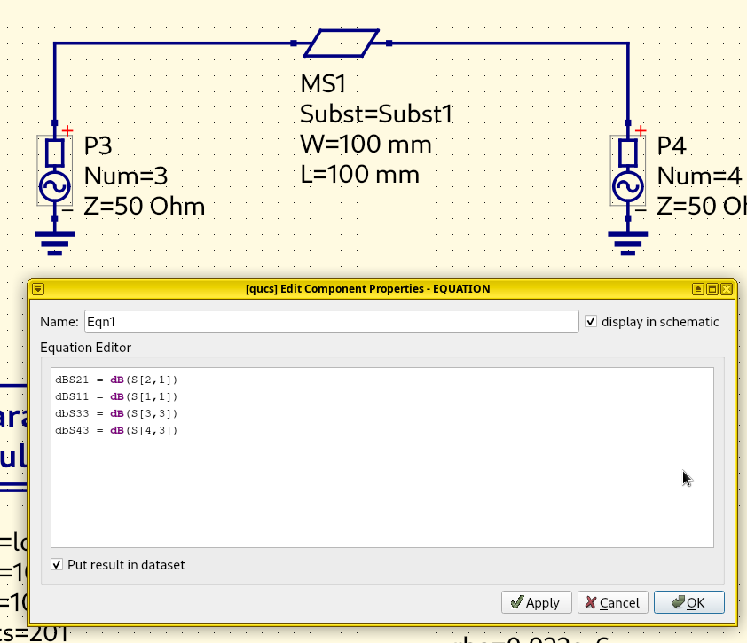
Change its formulas to the following:
dBS21 = dB(S[2,1])
dBS11 = dB(S[1,1])
dBS33 = dB(S[3,3])
dBS43 = dB(S[4,3])
Important
Make sure S[3,3] and S[4,3] matches the actual port numbers
on the schematics. If ports have been repeatedly deleted and inserted
into the schematic, they could be renumbered. If so, change the
port numbers back to 3 and 4.
Run simulation. Select Simulation and click Simulate. A dialog should pop up without warnings or errors.
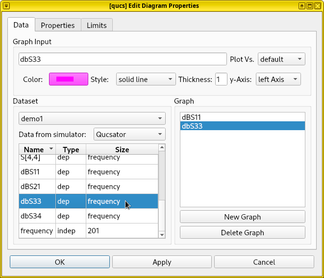
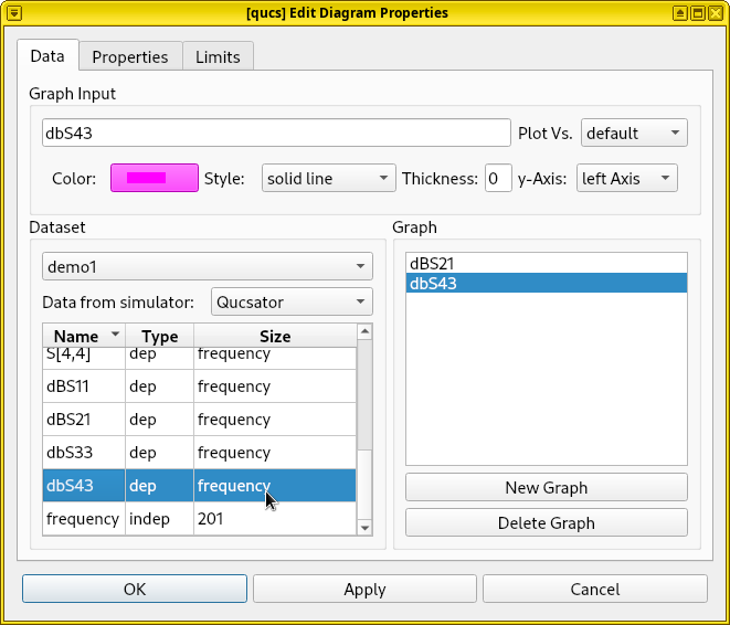
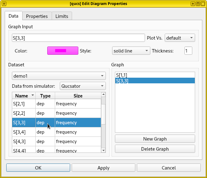
Plots. Double-click the original \(S_{11}\) chart, add dBS33 to the graph by double-clicking this item. Similarly, do the same to add dbS41 to the original S_{21} chart, and finally add S[3,3] to the Smith chart.
Results. By setting this Qucs-S simulation, we can compare the frequency response of a parallel-plate waveguide against a microstrip transmission line. From the simulation result, we find that their behaviors are significantly different. Both transmission lines have a resonance at 1.5 GHz, but their similarity ends here. At high frequencies, this parallel-plate waveguide has extremely high losses, while the microstrip transmission line is lossless.
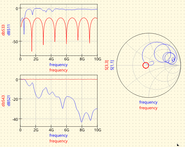
We will discuss the significance of this result at the end of this tutorial.