Boundary Conditions

In computational electromagnetics, all physical phenomena occur in a small simulation box, so we must decide what happens to the electromagnetic fields at its edges. These are known as the boundary conditions of Partial Differential Equations (PDEs). To create an effective simulation, we must select the appropriate boundary conditions. There are six in total, located at the six faces of the box: x_min, x_max, y_min, y_max, z_min, z_max. Each is independently adjustable.

Set Boundary Conditions

To set the boundary conditions of the simulator, use openEMS.openEMS.SetBoundaryCond() of the openEMS class. Its syntax is: SetBoundaryCond(bc) where bc is a list with 6 elements with the order of [x_min, x_max, y_min, y_max, z_min, z_max]. Each element is a string or integer according to the following table. Note that the use of integers is discouraged due to poor readability, but one may encounter them in older examples.

Boundary Condition	String	ID	Notes
Perfect Electric Conductor	`PEC`	0	Reflective. Fast.
Perfect Magnetic Conductor	`PMC`	1	Reflective. Fast.
Mur’s Absorbing Boundary	`MUR`	2	Absorbing. Slow. Best only for waves orthogonal to boundary with a known phase velocity (\(c_0\) by default). Named after Gerrit Mur.
Perfectly Matched Layer	`PML_8` `PML_x`	3	Absorbing. Slowest. `x` has a range [6, 20], 8 by default. Occupies `x` mesh lines near the boundary. Keep structures `x` cells away from boundary. For radiating structures, λ / 4 away.

Example

fdtd = InitFDTD();
bc = {'PML_8' 'PML_8' 'PML_8' 'PML_8' 'PML_8' 'PML_8'};
fdtd = SetBoundaryCond(fdtd, bc);

fdtd = openEMS.openEMS()
bc = ["PML_8", "PML_8", "PML_8", "PML_8", "PML_8", "PML_8"]
fdtd.SetBoundaryCond(bc)

Reflecting (Dirichlet) Boundary Conditions

If the finite nature of the simulation box and the reflection of EM waves at the boundaries are acceptable, reflecting boundary conditions offer a simple zero-overhead solution. They efficiently model structures inside metal enclosures, above a ground plane, or with an electric or magnetic field symmetry across a plane. No explicit modeling is necessary; the boundary conditions implicitly enforce these behaviors.

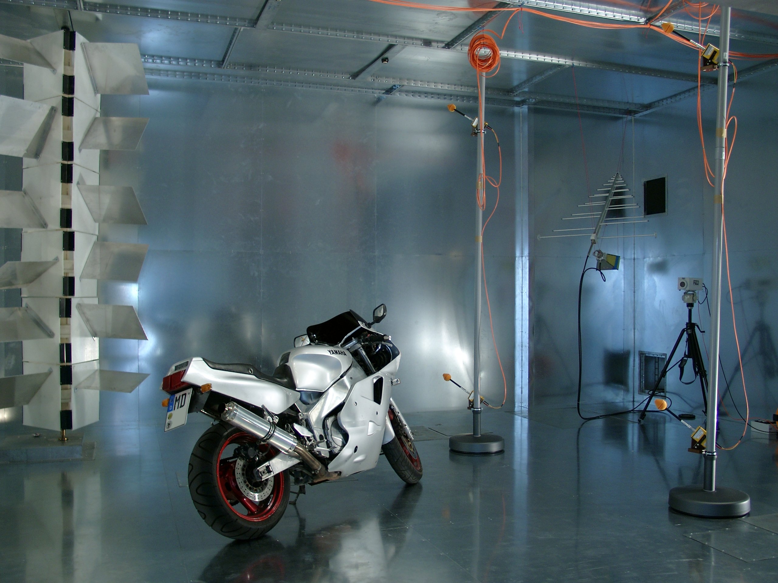
../_images/reverberation_chamber.jpg — A simulation box with PEC at all boundaries acts like a shielded enclosure. EMC test labs use room-sized metal enclosures to create reverberation chambers. Taking advantage of the standing waves due to reflections, one can create strong electric fields at localized regions to generate electromagnetic interference for testing. Image by Dr. Hans Georg Krauthäuser (Hgk at English Wikipedia), licensed under CC BY-SA 3.0.

Perfect Electric Conductor (PEC): The simplest treatment sets the (tangential) electric field at the boundary to 0. Since the electric field lines can’t penetrate this boundary, it’s equivalent to a Perfect Electric Conductor (PEC) with infinite conductivity \(\kappa\), also known as an Electric Wall. All incoming waves are fully reflected back, analogous to a 1D transmission line terminated by a short circuit.

Perfect Magnetic Conductor (PMC): By duality, it sets the magnetic field to 0 at the boundary. It acts as a boundary at which the magnetic field lines can’t penetrate. It’s equivalent to a Perfect Magnetic Conductor (PMC) with infinite conductivity \(\sigma\) (see Magnetic Conductivity), also known as the Magnetic Wall. All incoming waves are fully reflected back as well, but with a phase opposite to that of the PEC, analogous to a 1D transmission line terminated by an open circuit. It’s used mainly as a mathematical tool to enforce field symmetry when simulating a half-structure, as no natural material in the real world behaves like a PMC.

Mathematically, both PEC and PMC are Dirichlet boundary conditions that enforce fixed field values (e.g. zero).

Note

For our simulation, instead of explicitly modeling metal plates, we can model a vacuum with nothing inside, taking advantage of the PEC boundary conditions at z_min and z_max for fast computation. However, this is out of this tutorial’s scope, and it won’t capture the fringe fields above and below. We won’t use PEC or PMC in this example.

Absorbing Boundary Conditions (ABC)

In open-boundary problems, such as antennas or structures with radiation loss, Absorbing Boundary Conditions (ABC) must be used to suppress reflections to prevent spurious simulation results. At its boundaries, the electromagnetic waves are absorbed and dissipated without reflecting back, creating the illusion of an infinitely large free space. If PEC and PMC are analogous to a shorted or opened transmission line, the ABC is analogous to a termination resistor.

In general, these simulations should use a simulation box larger than the structure to avoid intrusion of strong fringe fields at the boundary. However, deliberately running a transmission line into the PML (defined below) can be used as a perfect termination. This allows one to terminate a transmission line without knowing its characteristic impedance, enabling impedance measurement. In fact, openEMS’s microstrip ports don’t create a lumped termination resistor by default, expecting users to place them into the PML at boundaries.

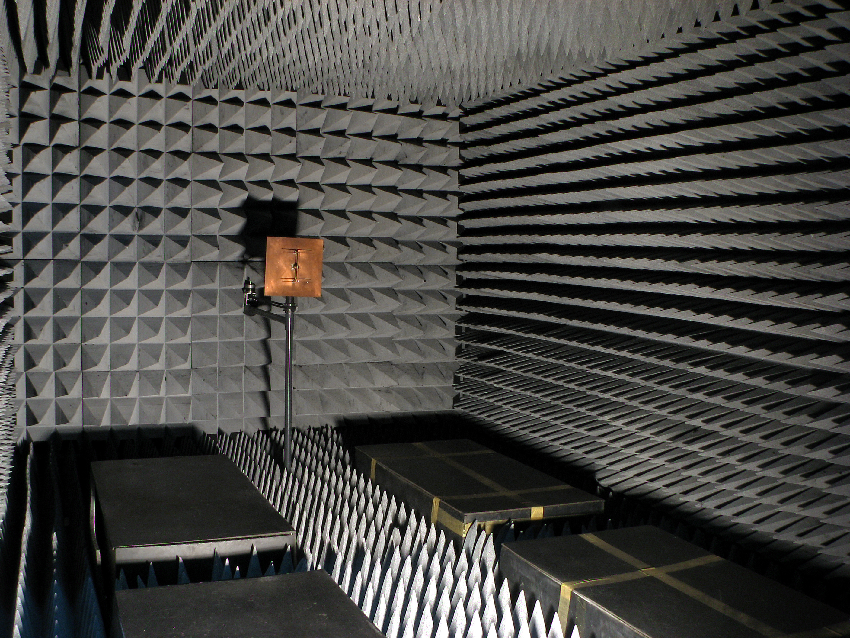
../_images/anechoic_chamber.jpg — A simulation box with PML at all boundaries acts like an anechoic chamber in an EMC test lab, mimicking an infinitely large free space. Image by Adamantios (at English Wikipedia), licensed under CC BY-SA 3.0.

Two kinds of Absorbing Boundary Conditions are implemented in openEMS.

Mur’s Boundary Condition (MUR). This is a first-generation boundary condition purely defined by differential equations, originally invented by Gerrit Mur in the 1980s, with a moderate computational overhead. It works optimally when the EM wave is traveling at a direction orthogonal to the boundary, at a known phase velocity. However, it’s less effective if a wave’s incident angle is oblique, or if the boundary’s phase velocity parameter differs from the actual EM wave. Imperfect absorption contributes to simulation errors.

See also

By default, Mur’s phase velocity parameter is set to the speed of light in free space. It may be adjusted via SetBoundaryCond()’s optional argument MUR_PhaseVelocity. For Python, this API is currently unimplemented.
Perfectly Matched Layer (PML). This is the second-generation boundary condition proposed in the 1990s, modeling the behavior of a hypothetical EM wave-absorbing material. Unlike Mur’s ABC, PML occupies some physical cells in the simulation box (the actual boundary at the true edge remains PEC). This mimics the wave-absorbing foam on the wall of an anechoic chamber in EMC test labs.

PML is a more effective absorber and is easy to use, but it has the highest computational overhead (especially in openEMS, due to suboptimal implementation). Avoid it if efficiency is critical (e.g. only use PML at the simulation box’s face directly hit by radiation, and use MUR for other boundaries). Intrusion of fringe fields and evanescent waves into the PML can destabilize it, causing the simulation to “blow-up”. Radiating structures must be kept at a distance of \(\lambda / 4\).

Important

In openEMS, PML_8 is commonly used, meaning the nearest 8 mesh lines of the simulation box are dedicated to the PML. This is an assumption made by the simulator and not visible in AppCSXCAD. Ensure your structures do not overlap with edge cells (unless intentionally terminating a region with the PML). As a rule of thumb, keep radiating structures at a distance of \(\lambda / 4\) from PML, as intrusion of evanescent waves (fringe fields) can create numerical instability. When in doubt, make a secondary simulation with the PML further away. If nothing changes, the original clearance was sufficient.