Field Dumps Analysis via ParaView

ParaView is a visualization program commonly used in the High-Performance Computing (HPC) and scientific computing world. One can install it using the operating system’s package manager.

In openEMS, we rely on ParaView to visualize raw electromagnetic fields created during the simulation. For troubleshooting malfunctioning simulations or understanding the physical behavior of a structure, this is especially helpful as one can identify the problematic region directly by visualization.

We continue our total current density visualization example, introduced as an optional step in fielddump. If the simulation finishes with field dump enabled, a series of vtr files (which is a type of the VTK file format) is created under the simulation directory.

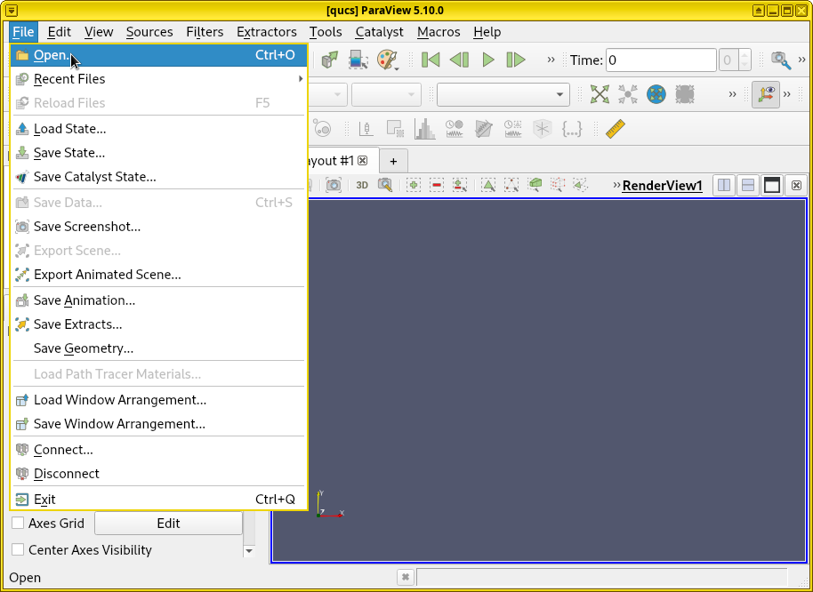
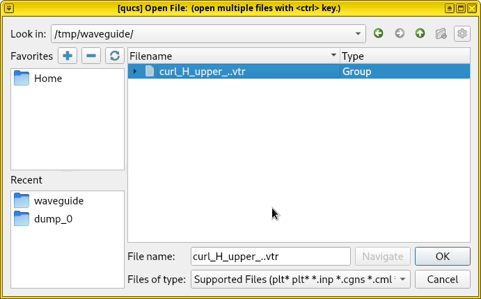
Open ParaView. To visualize these results, open ParaView first. Click Files ‣ Open. Navigate to the simulation data directory, open the vtr file series.

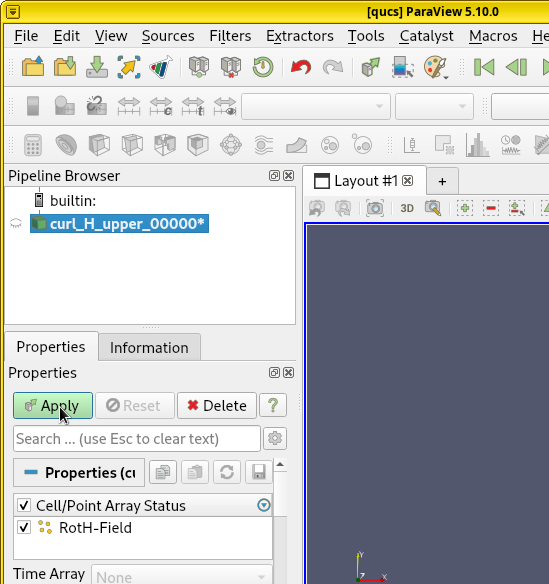
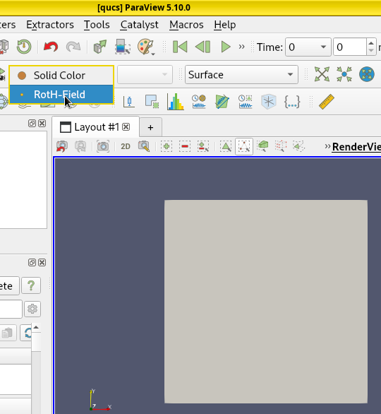
Apply cell/point array for visualization. Make sure RotH-Field appears in the Cell/Point Array list on the bottom left of the ParaView window, and is checked. Click Apply. By default, the visualization shows an empty rectangle because the displayed physical quantity is set to Solid Color without any data. Click Solid Color and change it to RotH-Field.

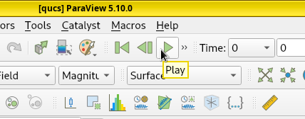
Play animated visualization. Now it’s possible to see the current density by clicking the Play button to see an animated visualization of electromagnetic wave propagation.

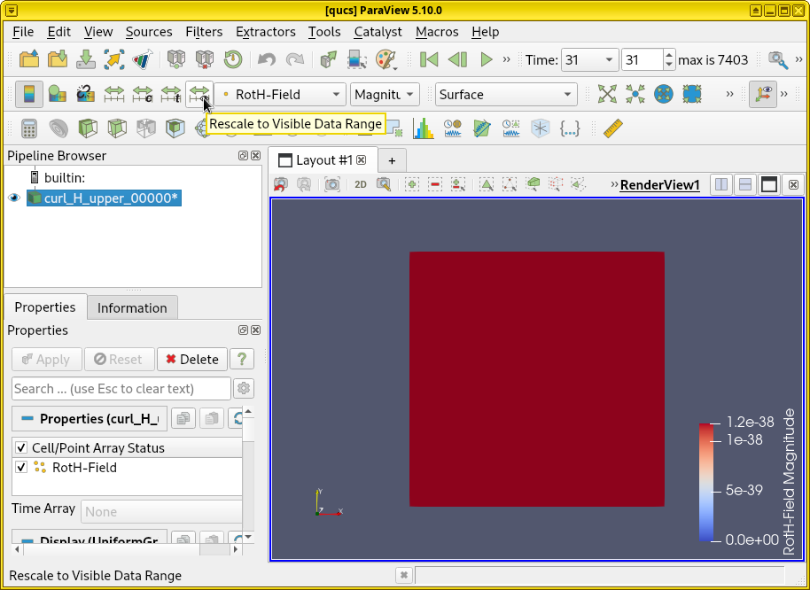
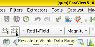
Rescale the color-grading. However, ParaView can still render this field dump incorrectly due to a problem in color-grading. If ParaView’s color-grading scale uses a small values for reference (as the field at t = 0 is zero), all fields (or current) injected by the excitation source in later timesteps can be rendered as a deep red as the color saturates, making them indistinguishable. This happens by default, as shown in the following diagram. We can solve this problem by clicking Rescale to Visible Data Range.

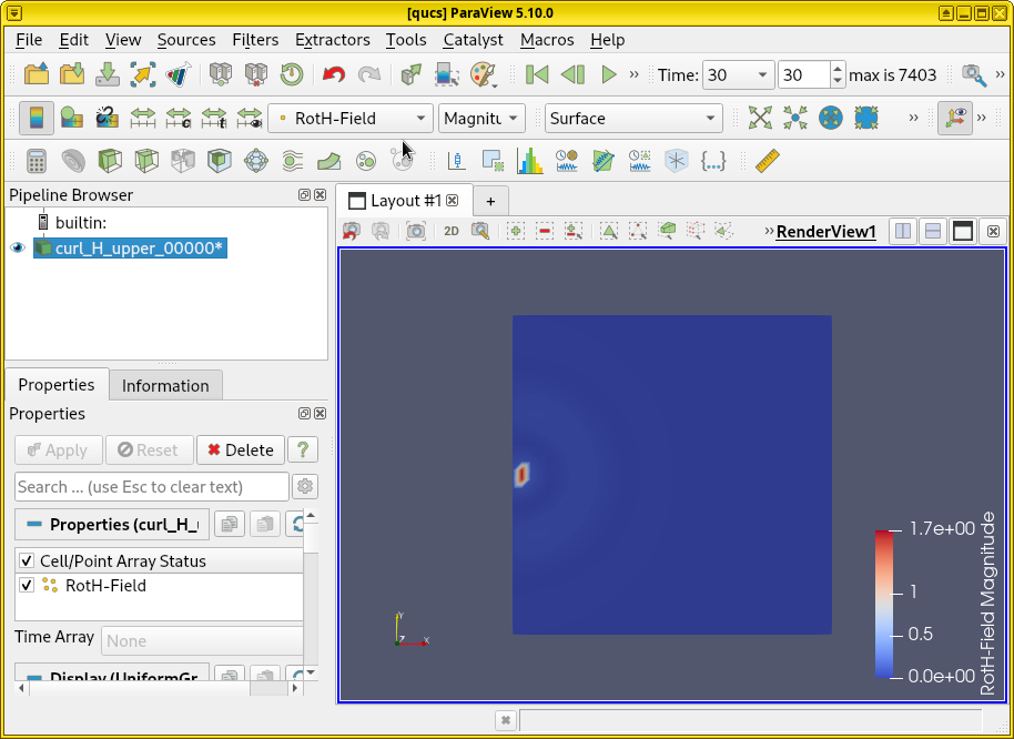
Color scale sensitivity to timestep. On the other hand, if large values are used for references, the beginning of the visualization works okay. But in later timesteps, colors will be very shallow and difficult to see. Thus the color-grading scale is quite sensitive to the timestep at which the Rescale to Visible Data Range button is pressed.

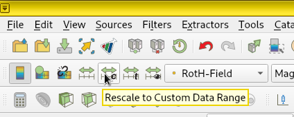
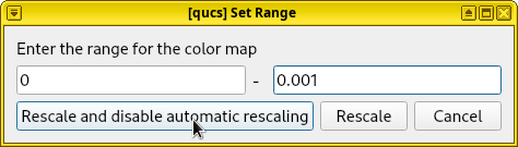
Manual color scale. Another problem is that the excitation port always have strong fields and currents, so as long as ParaView’s color-grading is normalized to the magnitudes around a port, all currents and fields at other locations may appear dark and weak. Thus, manually overriding the color-grading may be necessary. To do so, press Rescale to Custom Data Range, enter a new value (such as 0.001) and press Rescale and disable automatic rescaling.

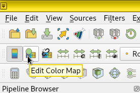
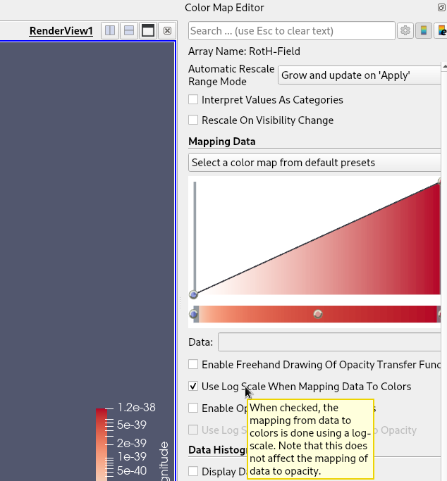
Logarithmical color scale. For good visualization, an alternative solution is to color-grade the values logarithmically. It can be done by clicking Edit Color Map. In the Color Map Editor on the right, check Use log scale when mapping data to colors. A warning message may immediately appear, as the log of 0 is undefined, but it’s safe to ignore.

Result. In this simulation, we find that rescaling at timestep 55 and enabling logarithmical color map allow us to obtain a satisfactory video below.

Important

To correctly visualize the fields in ParaView, one must apply the corresponding Cell/Point Array, select the variable that represents the physical quantity, rescale the color-grading (and optionally enable logarithmical scale) to match the data range. Otherwise, an empty box appears when the array is not selected. A solid color appears when the color map’s data range is saturated.

Also, 3D dump boxs are tricky to visualize. By default it’s rendered as an empty box. It’s possible to render a 2D slice of the data, or possibly a 3D vector field. But it’s beyond the scope of this tutorial.